DOI: http://dx.doi.org/10.18180/tecciencia.2013.15.9

System and Software Development to Measure Cylindrical Pipes Based on Acoustic Reflectometry

Sistema y desarrollo de software para la medición de tubos cilíndricos basado en la reflectometría acústica

Marcelo Herrera Martínez¹, Andrea Gualtero Mosquera², Raúl Enrique Rincón Flórez³

1. Universidad de San Buenaventura, Bogotá, Colombia, Mherrera@usbbog.edu.co
2. Universidad de San Buenaventura, Bogotá, Colombia, agualtero@academia.usbbog.edu.co
3. Universidad de San Buenaventura, Bogotá, Colombia, Rrincon@usbbog.edu.co

Received: 17 May 2013 - Accepted: 28 Oct 2013 - Published: 30 Dec 2013

Abstract

The following document describes the use of the acoustic reflectometry, the theory that follows it, and its implementation as a technique to measure cylindrical pipes. It describes how it was constructed and the materials used in the construction and implementation of the system that allows capturing signals (reflections) from the pipe under evaluation; also shown herein are the results obtained from measuring pipes of different lengths. This work also proposes simple application software that allows analyzing measurements made using acoustic reflectometry, as well as some conclusions and recommendations for future work.

Keywords: Measurements, Acoustic Reflectometry, Cylindrical Pipes.

Resumen

El siguiente documento describe el uso de la reflectometría acústica, la teoría en la que se basa, y su implementación como una técnica para la medición de tubos cilíndricos. Se describe la manera y los materiales utilizados en la construcción e implementación del sistema, denominado reflectómetro, que permite la captura de las reflexiones provenientes del tubo bajo medición. También es propuesto un software de aplicación sencillo que permite el análisis de las mediciones realizadas utilizando la reflectometría acústica y algunas conclusiones y recomendaciones para trabajos futuros.

Palabras clave: MATLAB, Mediciones, Reflectometría Acústica, Tubos Cilíndricos.

1. Introduction

Acoustic reflectometry is a non-invasive technique based on the capture and later analysis of reflections produced by impedance changes in cylindrical pipes. It has been used to analyze wind musical instruments, given that it can furnish information on the object’s geometric characteristics and acoustics. Recent studies propose it as a technique that offers precise measurements in pipe diagnosis, basing all analyses on the behavior of sound waves that propagate with a flat wave front.

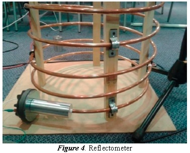
This study is about the measurement and later analysis of cylindrical pipes by using acoustic reflectometry. A capturing system was constructed and implemented denominated reflectometer. Analysis was performed of the reflections captured to determine what important information can be obtained from these measurements.

The measurements made by using this technique permit knowing the pipe’s input acoustic impedance, as well as its length and the possible identification of leaks or obstructions in it. The results of this project serve as a foundation and provide guidelines to conduct subsequent studies requiring acoustic analysis of musical instruments, and diagnosis of pipes. Also, limitations were identified and analyzed in the use of this technique as in the information that can be obtained from measurements made of cylindrical objects.

2. Background

Research on acoustic reflectometry and its different applications has been conducted for some considerable time. Many well-developed studies have been made on its application when characterizing wind instruments, which are, per se, cylindrical pipes. These studies have demonstrated that input acoustic impedance measurements (which provide valuable information on the wind instrument under evaluation) made by using acoustic reflectometry are quite close to theory and easily applied; likewise, having some restrictions in the information obtained at high frequencies and in the size of the reflectometer, which is of considerable length [1].

Additionally, experiments and research has been conducted on the use of this technique to identify leak detection and obstructions in pipes [2], which would be of great use at industrial levels in the area of preventive and corrective maintenance. In this sense, studies have also been carried out on the characterization and identification of joints between pipes, like: “Tee”, elbow, and semi-elbow joints; pipe end – open or close, among others . This characterization of joints, as well as the identification of leaks and obstructions, demonstrates the possibility of using acoustic reflectometry in a more industrial setting. [3]

3. Theoretical framework

Acoustic reflectometry is the measurement of reflections from a pipe under evaluation, which are produced by impedance changes. Bearing in mind that the impedance of a cylindrical pipe depends on and is inversely proportional to its cross-section area, Z = p₀c/A, every time there is a change of area an impedance change will be produced, hence, part of the sound wave will be transmitted and part will be reflected, with these reflections captured and analyzed by using acoustic reflectometry. Also, the whole analysis and theory upon which this technique is based is on the propagation of unidirectional sound waves, that is, with a flat wave front.

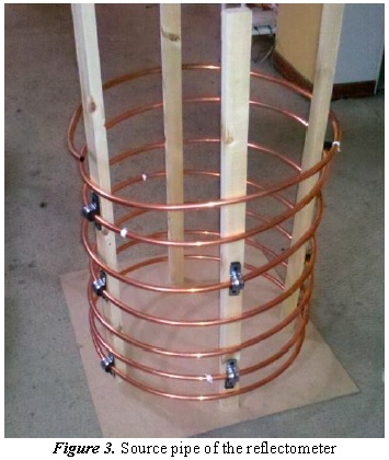
The following details the measuring procedure made. An acoustic signal is released, ideally an impulse, through an electro-acoustic transducer. This signal travels through a pipe called source pipe, which must have a determined length depending on the pipe length that will be measured. When the signal reaches the pipe under evaluation, a set of reflections will be produced that are, per se, its impulse response. The reflectometer scheme is shown in Figure 1 [1].

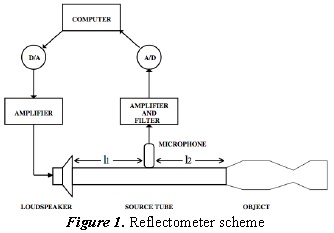
The L₂ section of the source pipe must be long enough to make sure the impulse has passed completely before the first reflections reach the microphone. On the other hand, the L₁ section of the source pipe must be long enough to separate and make sure the microphone manages to capture the reflections from the object before these reflections, which continue their path back through the source pipe, are again reflected with the loudspeaker and again reach the microphone, producing contamination and hindering the identification of reflections coming only from the pipe under evaluation.

3.1. Input acoustic impedance from the impulse response

The input acoustic impedance of a cylindrical pipe provides valuable information on its behavior within the frequency domain. This can be calculated from the impulse response measured of the object being evaluated.

The sound pressure at the limit between two different areas within a tubular object is the sum of the incident wave and the reflected wave. Likewise, this applies to the volumetric rate, but, with a negative sign because it is a vector and it must specify the propagation direction. Having as incident signal the input signal to the system, that is, an acoustic impulse, and as reflected signal, the object’s impulse response (reflections); and bearing in mind that the acoustic impedance is the ratio between pressure and volumetric rate, we may relate the impulse response to the impedance, as shown ahead.

Impedance (Z) is the ratio between pressure (P) and volumetric rate (U)

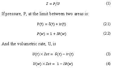
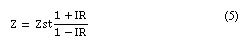
Where Zst is the impedance of the source pipe. It is replaced in equation 1 to obtain the impedance of the pipe under measurement from the mean impulse response.

3.2. Reflection coefficient at the limit between two surfaces [1]

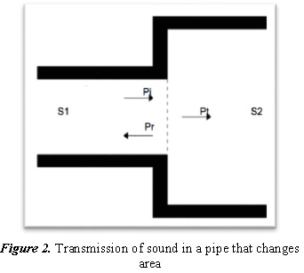
Bearing in mind Figure. 2 and placing equation 4 in the following terms:

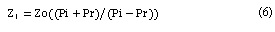
Where:

Pi: Incident wave
Pr: Reflected wave
Zo: First section impedance
Z1: Second section impedance

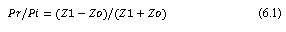
Clearing Pr/Pi, we have the reflection coefficient in terms of impedance.

Bearing in mind that the impedance of a pipe is Z = p₀c/A is replaced to obtain the reflection coefficient in terms of areas 1 and 2.

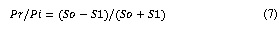
Thereby, if area two is bigger, the reflection coefficient will be negative, and if area two is smaller, it will be positive.

3.3. Theoretical input acoustic impedance of a cylindrical pipe with open end [4]

The acoustic impedance in cylindrical pipes depends on some of their characteristics, like length, behavior of the area along the whole length, and type of end. Pipes resonate at specific frequencies that propagate in flat manner.

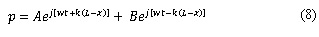
The pressure along the pipe of length x = L and of cross-section area S is given by the following equation:

Remembering that impedance is the ratio between pressure and volumetric rate, which is a vector, we obtain the impedance in x = 0 and in x = L

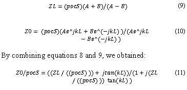
Where ZL for a pipe with open end is equivalent to its radiation impedance, given that it releases the sound to the environment. For a pipe with open and free end this impedance is given by:

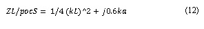
Where a is equal to the pipe radius.

Upon illustrating the input acoustic impedance of a pipe within a broad range of frequencies, an impedance curve is obtained. The acoustic impedance curve reveals the pipe’s resonance and anti-resonance frequencies. The lowest values are equivalent to the resonances and the highest values correspond to anti-resonance frequencies.

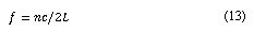
The resonance frequencies of an open pipe are given by the following equation:

Resonant harmonics will be present if the wavelength of the frequency released is much greater than the pipe radius through which they are being transmitted; that is:

4. Design and construction of the reflectometer

For the source pipe, a flexible copper pipe 13 mm in diameter was used, through which, according to equation wc=1.84c/radio, the frequency as of which the waves will not propagate flatly is approximately 15 KHz. It will be shown ahead that there is large energy loss at high frequencies; besides the aforementioned, because of the distance that must be travelled, which is significant.

Lengths L₁ and L₂ of the source pipe designed are 8.5 and 3 m, respectively. This ensures, first, that the first group of reflections will reach the microphone after the input signal passes through it completely. Secondly, that up to four groups of secondary reflections could be captured, thus, managing physical isolation (in time) among the reflections of the object being measured and the reflections that will be present through the loudspeaker. Considering this, the object being evaluated could have a maximum length of L₁/n [1], where n is equal to the degree of secondary reflections that can be isolated. For our case, the object’s maximum length is 2 m, with n equal to 4.

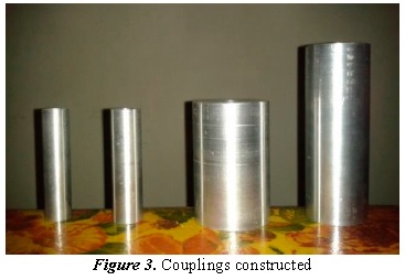
For the system (reflectometer) it is vitally important to transmit the input signal without losses, since its exit from the loudspeaker to its arrival at the object being measured. Due to this, couplings must be used to permit joining the different parts of the reflectometer. These couplings should minimally alter the object’s input signal and reflections. Couplings were constructed from aluminum bars, according to recommendations made by previous research [1]. The couplings were made as smooth as possible to avoid any reflection, and to make sure the change of area was not abrupt, but gradual. Couplings were made to permit the junction between the loudspeaker and the source pipe, and between the source pipe and the different pipes measured.

The PRV D280-Ti compression motor (driver) and the Tef 04 measurement microphone – because of its flat response – were used as input and output transducers. Ahead, it will be shown why using this type of output transducer is perhaps not the most adequate. Also, the Presonus FireStudio Mobile audio interface and the Alesis 150 power amplifier were used.

4.1. Measurements

As input signal, a logarithmic sine frequency sweep was taken along with a pulse, which was a wave squared with a useful time cycle equal to t₁=1/2fmax, where fmax is the highest frequency it will contain. To generate these two input signals used, Adobe^® Audition^® 3 and plug in Aurora software were implemented.

The sampling frequency used in all measurements was Fm = 44100 Hz. The sine frequency sweep was from 100 to 16 Hz with 25-second duration [3].

The calibration signal was captured finishing the source pipe with a 5-mm thick acrylic film. Capturing this reflection will permit deconvolution with the reflections of the measured pipe and, thus, remove the information provided by the source pipe [3]. This procedure will make the input acoustic impedance more exact.

4.2. First measurement

The first measurement used a pulse as input signal. Herein, we used three smooth PVC pipes 15 mm in internal diameter, each measuring 1, 0.5, and 0.12 m. Each of these pipes had two configurations, with their final end open and closed; yielding a total of six configurations, two per length. Measurement of each configuration was repeated 10 times to determine how much one measurement varied from another, in order to verify the fidelity of the system constructed.

4.3. Second measurement

The second measurement was made of seven smooth PVC pipes, of different lengths and with four configurations (final end open, closed, “Tee” end, elbow end, and semi-elbow end). Each take was done only once per input signal (sine sweep and pulse). The two input signals, impulse, and sine frequency sweep were used.

This measurement was made to test the precision of the constructed measurement system, comparing the length measured with a tape meter, and the measurement made by using acoustic reflectometry. The lengths of the pipes measured were 1, 0.5, 0.35, 0.18, 0.12, and 0.08 m.

4.4. Analysis of results

The microphone placed at a distance L₂ from the end of the source pipe captures the input signal when it passes through the microphone and the reflections of the pipe being measured. These reflections are the impulse response from the pipe being measured, which is why they provide information about it.

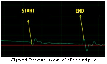
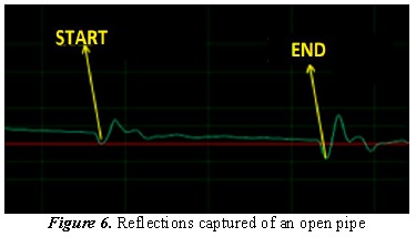
Upon observing what has been captured, we can clearly identify the start and end of the pipe under evaluation. In turn, it is possible to calculate its length by measuring the length in samples from peak to peak of each reflection. To convert it to meters, the following ratio is kept in mind:

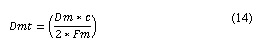
Where Dm is the distance in samples, c is the rate of the sound in the air, and Fm is the sampling frequency at which the measurements were recorded; divide by two because the signal must travel the same distance twice.

There is another important characteristic that can be seen in the two previous figures, the phase from the second reflection, that is, the reflection produced at the end of the pipe. This reflection has a negative peak if the pipe has an open end; or a positive peak if it has a closed end. This due to what has been previously explained on the reflection coefficient at the limit between different areas.

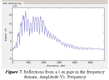
On the behavior of the measurements in the frequency domain, a drastic loss can be observed from approximately 2500 Hz, and before approximately 800 Hz. The loss at low frequencies is due to the output transducer used, which starts to have good performance at 900 Hz. Loss at high frequencies is due to the big distance the wave must travel, which is over 11.5 meters; this energy loss mainly affects high frequencies.

4.5. Analysis of the first measurement

The results of this measurement, previously described, demonstrate the system’s fidelity; understanding as fidelity when a device always yields the same data if measuring the same object.

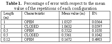
Using equation 13, distance in meters of the pipe being measured was calculated for each of the repetitions. Already having this measurement, we proceeded to calculate the percentage of error with respect to the total mean value of the repetitions per configuration. Very low percentages of error were obtained, as noted in Table 1. The percentages of error shown in Table 1 confirm that the measuring system based on acoustic reflectometry will show approximately the same results (mean pipe length) if the same object is measured several times.

4.6. Analysis of the second measurement

This measurement compared the value measured in meters of the peak-to-peak distance between reflections to the real value (value measured with a measuring tape). This was done to test how much the reflectometer failed to measure the pipe distance.

The following figure shows the comparison and the percentages of error obtained with both input signals (pulse and sine frequency sweep).

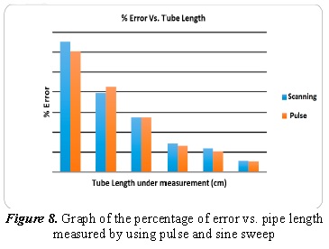
It is clearly noted that the shorter the pipe being measured, the higher the percentage of error will be, leading to very high values. This is because in short pipes the reflections contaminate each other, thus, hindering the identification of the pipes.

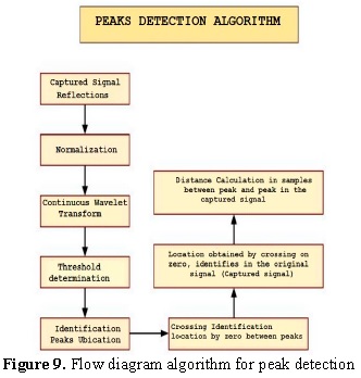
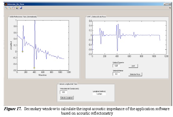
4.7. Algorithm for peak detection

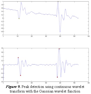
For approximate calculation of the pipe length measured by using acoustic reflectometry, an algorithm was written in MATLAB to detect the location of the peaks corresponding to the reflections from the pipe being measured. The algorithm follows the flow shown in Figure 9. The algorithm uses continuous wavelet transform (cwt), given that analysis of non-periodic signals, as in this case, through wavelets is more complete and precise. Different wavelet functions were experimented with, finally opting for the Gaussian wavelet function because it behaved best and permitted more easily identifying these peaks.

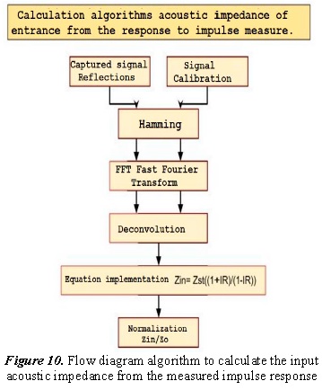
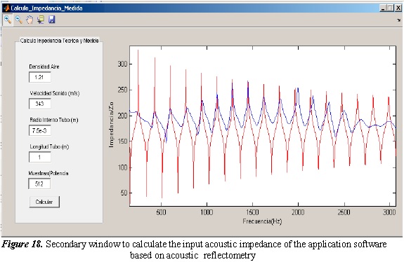
4.8. Input acoustic impedance from the measured impulse response

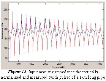
The algorithm written to calculate the input acoustic impedance from the measured impulse response was conducted in MATLAB and follows the flow shown in Figure 12.

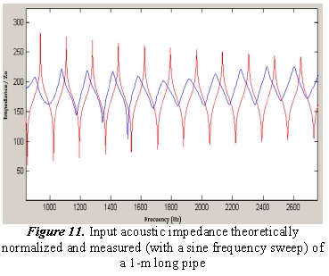
The impedance curves obtained through this algorithm (blue) and the comparison to the theoretical curves (red) are shown ahead. Figures 11 and 12 show the comparison between the measured and theoretical acoustic impedances for a 1-m pipe. The measured impedance is not exactly equal to the theoretical, given that to calculate the theoretical losses and aspects like pipe material, wall thickness, transducers used, among others are not kept in mind. Besides the aforementioned, the measurement does not have information on very high frequencies due to the energy loss present in them, and at frequencies below 1 Khz the information is also not reliable; this is because the output transducer is a compression driver and these start to better operate at 900 Hz, as had been discussed previously. Although the measurement is not exactly the theoretical, it provides a very close idea of which are the pipe’s resonance frequencies.

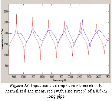
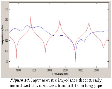
Because of these losses at high frequencies, the shorter the pipe being measured less exact will be the input acoustic impedance measured. This is because in shorter pipes the resonance frequencies are higher and in the measurements made this information was not found. Figures 13 and 14 show the acoustic impedance measured against the theoretical acoustic impedance of a 50-cm pipe and an 18-cm pipe, respectively.

5. Application of software in Matlab

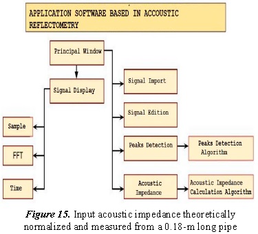
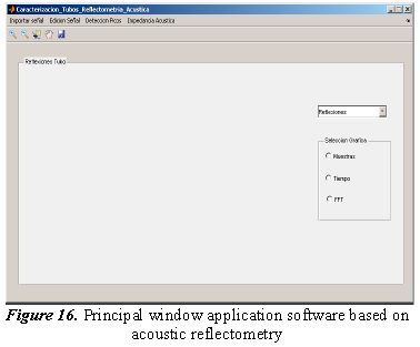
Bearing in mind the reflectometry theory and the relationship between a pipe’s impulse response and its acoustic impedance, an application was developed to analyze the signal captured by the microphone on the reflectometer and, thus, reveal a geometric characteristic like the pipe length, and an acoustic characteristic like input impedance of the objects being measured.

The application was developed in MATLAB, given that it has commands and functions that facilitate the development of mathematical algorithms. The application implements the algorithms previously described to detect peaks, approximate calculation of the pipe length, and calculation of the acoustic impedance from the signal captured in the measurements. An interphase graphic is available with a principal window that has the menu which permits performing the different available actions. These actions are: import the signals, visualize them in different domains (frequency, time, and samples), editing the signals, and access to windows of peak detection and acoustic impedance. The following figure shows the options and access available from the principal window.

The following show the images of the application windows.

6. Conclusions

To emit the input signal, it is not necessary for the output transducer (loudspeaker) to have a flat response at very high frequencies, given that independent of the transducer used, these will be attenuated and reliable information cannot be obtained from a mere 3 KHz.

Calculation of the acoustic impedance from impulse response is simple and provides results that are quite close to theory. Its precision with respect to the theory is affected by the signal-noise ratio present, the energy loss at high frequencies, and the material characteristics of the pipe being measured.

The system constructed permits known the approximate length of the pipe being measured. Measurements are more precise with longer pipes, obtaining approximately 5% error percentage for pipes between 50 and 100 cm, meaning that the system has a 5-cm error for every meter. Measurement precision for object length diminishes for shorter pipes.

To make better measurements, the audio interface must be high end, with enhanced A/D converters and better pre-amplifiers. The signal should be altered the very least possible by these elements. Data acquisition cards should be used to capture the signals.

Acoustic reflectometry could be used to identify leaks or obstructions in cylindrical pipes, given that depending on area changes the reflection phase changes.

7. Considerations for future work

The following will be considered for future work:

Use of another input signal like MLS, which provides better signal-noise (S/N) ratio.

Implementation of an impulsive input signal generated electrically. This signal is closer to a Dirac delta function, δ(t), and is not affected by a reproduction and transduction system.

Use a data acquisition card that permits samples at higher sampling frequency and permits saving the data in a computer, and design an instrumentation preamplifier to diminish electronic noise.

Suggest the possibility of measuring acoustic silencers, from reflections captured or from the input impedance measured.

References

[1] D. B. Sharp, Acoustic pulse reflectometry for the measurement of musical wind instruments. For PhD., Edinburgh: University of Edinburgh, 1996.         [ Links ]

[2] D. B. Sharp y D. M. Campbell, «Leak detection in pipes using acoustic pulse reflectometry,» Acta Acustica united with acustica, vol. 83, nº 3, pp. 560-566, 1997.         [ Links ]

[3] A. Kestian, A new junction identification method utilizing acoustic reflectometry, New York: The Steinhardt School, New York University, 2007.         [ Links ]

[4] L. Kinsler, Fundamentals of Acoustics, New York: Willey, 1996.         [ Links ]