DOI: http://dx.doi.org/10.18180/tecciencia.2014.16.1.

Techniques for alarm management with fault diagnostic system in startups and shutdowns for industrial processes

Técnicas para gestión de alarmas con sistemas de diagnóstico de fallas en procedimientos de arranque y parado de procesos industriales

Jhon William Vasquez Capacho¹, Manuel Alejandro Mayorga², Alexander Cortez³ Alexander Cortez⁴, Alvaro Bustos⁵

¹ Universidad de los Andes, Bogotá, Colombia,
w.vasquez10@uniandes.edu.co
² Escuela Colombiana de carreras industriales, Bogotá, Colombia, mmayorgab@ecci.edu.co.
³ Escuela Colombiana de Carreras Industriales, Bogotá, Colombia, alexandercort@gmail.com.
⁴ Escuela Colombiana de carreras industriales, Bogotá, Colombia,
vbernalt@ecci.edu.co.
⁵ Servicio Nacional de aprendizaje SENA, Bogotá, Colombia,
alvarobustos@misena.edu.co.

How to cite: Vasquez, J., et al., Technical for alarm management with fault diagnostic system in starups and shutdowns for industrial processes, TECCIENCIA, Vol. 9 No. 16., 9-21, 2014, DOI: /dx.doi.org/10.18180/tecciencia.2014.16.1.

Received: 02 March 2014 Accepted: 15 April 2014 Published: 30 July 2014

Abstract

This paper presents a preliminary study of the different techniques that can be used for fault diagnostics in industrial processes specially on the startup and shutdown procedures. A review of these techniques from the perspective of how its can be used for Alarm management is presented, followed by an analisys of fault diagnostic in complex systems passing techniques like the causal graph. Another technique exposed is the use of chronicles as a robust method for fault diagnosis; in a first part we examine aspects as diagnostic, Timed Diagnosability, then propose an automated translation of chronicles, and how it can be used on the alarm management in a starting or shutdown plant. Concluding with a preliminar methodology propoused that includes the use of the causal graph with the chronicles in an Alarm management.

Keywords: Alarm management, Causal Graph, Chronicle, Fault diagnostic, Timed diagnosis.

Resumen

En este trabajo se presenta un estudio preliminar de las diferentes técnicas que se pueden utilizar para el diagnóstico de fallas en los procesos industriales especialmente en los procedimientos de inicio y parado. Una revisión de estas técnicas desde la perspectiva de cómo se pueden utilizar para la gestión de alarmas es presentada, seguido de un análisis del diagnóstico de fallas en sistema complejos pasando a técnicas como la gráfica casual. Otra técnica expuesta es el uso de crónicas como un método robusto para el diagnóstico de fallas; en una primera parte se examinan aspectos como el diagnóstico, diagnosticabilidad temporizada, luego se propone un traslado automatizado de crónicas y la forma en que se puede utilizar en la gestión de alarmas en una planta, en el arranque o el apagado. Concluyendo con una propuesta metodológica preliminar que incluye el uso de gráfico casual con las crónicas para la gestión de alarmas.

Palabras clave: Gestión de alarmas, grafica casual, crónica, diagnóstico de fallas.

1. Introduction

The increasing automation of industrial production processes has resulted in an increasing complexity of control systems. These systems are based on digital technologies that requires them to increase their capacity in terms of the number of variables that can be treated, its processing speed and communication capacity [1]. In addition, on highly automated systems is an usual requirement automatic reconfiguration on embedded control system [2] [3] [4], and the ultimate goal is to optimize the availability, reliability and safety of production processes [3].

As result, Diagnosis and fault detection is an important problem in engineering process currently, and it is the central component of an abnormal events management (AEM), which has attracted much attention recently. AEM is responsible for the detection, diagnosis and correction of abnormal conditions and faults in a process [5]. Early fault detection and diagnosis in a process while the plant continues to operate in the controllable region and can help avoid abnormal events increase. Since petrochemical industries looses an estimated $ 20 billion in the U.S. alone each year, AEM has been classified as the number one problem that needs to be solved [6] [7]

Hence the alarm management is one of the aspects of great interest in the safety planning in the different plants [8]. Integrated management of the critical factors in the process ensure optimum reliability level in production [9]. Factors such as control of the process variables which are monitored from the computer systems that run the control algorithms and strategies especially in the strategies, procedures and steps followed in both startup and shutdowns and try to keep the plants within the operating established "limits" [10].

On a startup or shutdown process the quantity of signals provide how alarms increase, then the safety of a plant involves integrated management of many factors that matter most when analyzing the causes of the accidents [3] [11] [12] [13] [14] [15] [16] [17] [18]. In other words, these factors must be managed as joint, and not separately, because if any of them outside unattended or decreased, the security would be threatened [19]. The critical factors of the process work that must be managed together are:

- Facility safety.
- Control of process variables.
- Safe behaviors.
- Valid procedures.

This raises the need for a diagnostic system and operator prompting, so as to achieve a system that helps to maintain, thereby reducing diagnosis time, resulting in increased availability characteristic of installation. Then a chronicle, record or history of the sequence of the alarms could be fundamental for an efficient fault diagnostic [20]. After identifying the faults it is necessary that the process will recover automatically to ensure the efficiency of the system [21] and it is an important aspect specially for the industrial sector in his startup and shutdown procedures. We aim at presenting an exposition of some fault diagnostic techniques with the description of the Graph models and the Chronicles related with diagnosability. Followed by a preliminar methdology proposed where some of the techniques described are integrated.

2. Fault diagnosis methods

The need of developing safety in the industrial process has permited the fault diagnostic researches evolution. The fault diagnosis in general consists in the following three important aspects: Fault detection: discovery of the existence of faults in the useful units of the process, Fault isolation: localization (classification) of diferent faults, and Fault analysis or identification: determination of the type, degree and origin of the fault. To carry out a basic analisys of the fault diagnostic evolution it is necessary to review one of the first studies in fault diagnostic for electronic system; since the 50 years, followed by the 60' s, 80' s, 90' s and the current tendences.

In the first stage, the most reliable components were implemented on the first generation of electronic computers (1940 end in the mid-50s), therefore, practical techniques were used to improve reliability, and control codes of errors, duplex with comparison the tripling of the feedback, diagnostic locate defective components among others techniques. John Von Neumann [22], E. F. Moore and C. E. [23], and their successors established theories of using redundancy to build stable logic structures from less dependable components, whose faults were veiled by the presence of multiple redundant components [7].

The theories of masking redundancy were integrated by W. H. Pierce as the concept of failure tolerance in 1965 [24]. In 1967, A. Avizienis integrated masking with the practical techniques of error detection, fault diagnosis, and recovery into the concept of fault tolerant systems [25]. On the events the work on software fault tolerance was initiated by Elmendorf [26], later it was complemented by recovery blocks [27], and by N-version programming [28]. Then, the urge of a consistent set of concepts and terminology was accelerated by the formation of the IEEE-CS TC on Fault-Tolerant Computing in 1970 and of IFIP WG 10.4 Dependable Computing and Fault Tolerance in 1980.

In 1982 at FTCS-12 seven position papers were presented; in a particular session on elementary concepts of fault tolerance, and J.C. Laprie exposed a synthesis in 1985. additional work by members of IFIP WG 10.4, guide by Laprie, the book Dependability: Basic Concepts and Terminology [29] was concluded in 1992, in which the English text was also translated into French, German, Italian, and Japanese. In this book, intentional faults (hateful logic, intrusions) were listed along with accidental faults (physical, design, or interaction faults). Tentative research on the integration of fault tolerance and the defenses against deliberately malicious faults, i.e., security threats, was started in the mid-80's [30] [31] [32]. The first IFIP Working Conference on Dependable Computing for Critical Applications (DCCA) was held in 1989. This and the six Working Conferences that followed fostered the interaction of the dependability and security communities, and advanced the integration of security (confidentiality, integrity and availability) into the framework of dependable computing.

Since 2000, the DCCA Working Conference together with the FTCS became part of the International Conference on Dependable Systems and Networks (DSN) [25] [26] [28] [33] [32] [34] [35]. Venkatasubramanian proposes a diagnostic framework where it indicates the diferent sources of failures in it, but now we go to analyze the alarms, the time and the operators action to determinate a new framework for diagnostic. From an Alarm management perspective, some methods exists or techniques that require accurate process models, semi-quantitative models, or qualitative model. On the other hand, there are other methods that do not assume any form of model information and rely only on process history information. In addition, given the process knowledge, there are different search techniques that can be applied to perform diagnosis. Such as a collection of bewildering array of methodologies and alternatives which often pose a difficult challenge to any aspirant who is not a specialist in these techniques. Some of these ideas seem so far apart from one another that a non-expert researcher or practitioner is often left wondering about the suitability of a method for his or her diagnostic situation. While there have been some excellent reviews in this field in the past, they often focused on a particular branch, such as analytical models, of this broad discipline. There exists quantitative model based methods, qualitative model based methods, and process history based methods [7].

A wide diversity of techniques such as the early attempts using fault trees and digraphs, knowledge-based systems, neural networks, Process history information, causal graphs, analytical approaches, chronicles, time petri nets, in more recent studies are computer aided methods for the process fault diagnostic problematic that have been developed over the years. The Fault trees is a tool used to locate and to correct incidents. They can be used to prevent or to identify incidents before they happen, but they are used with more frequency to analyze accidents or such research tools that indicate faults. When happening oneself an accident or a fault, it can be identified the root cause of the negative event. In this diagrams the time is not involved. An expert system or knowledge based system can be defined as: "... system that solves problems using a symbolic representation of the human knowledge" [36].

Knowledge-based systems performance based on the quantity and quality of knowledge of a specific domain rather than in technical troubleshooting. Differences between knowledge-based systems and other techniques: In mathematics, control theory and computer, trying to solve the problem through its modeling (model problem). In an expert systems the problem is attacked by building a model of "expert" or problem solver (expert model); in the Alarm Management with fault diagnostic the human knowledge will be so important for defining the Failure mode of the equipment to analyze. Neural networks are a very important field within the Artificial Intelligence. An artificial neural network (ANN) can be defined as a directed graph with the following restrictions: The nodes are called processing elements (PE) [37].

The bonds are called instant connections and function as one-way paths. Each PE can contain any number of connections. All connections departing from an PE must include the same sign. The PE can contain local memory. Each PE preserves a transfer function which, depending on the local memory and the inputs produces an output signal and in some cases it transforms the local memory. The inputs to the ANN come from the outside world, while its outputs are connections leaving the ANN. For the Alarm management with fault diagnostic the theory of the ANN could be applied for training system on the reconigtion the units of time necessary in each chronicle. Process history information allows to the systems to detect deviations according to an a historical data base, but in a startup procedure this type of data is not found [4], [38], [39].

3. Model based fault detection

The model-based fault diagnosis technique is a method relatively new in the traditional engineering domain technical fault diagnosis, it had been developmented fast and now receiving significant consideration. The following approaches must be considered. First, the hardware redundancy based fault diagnosis: A fault in the process component is then detected if the output of the process component is diferent from the one of its redundancy. Second, the Signal processing based fault diagnosis: On the hypothesis that some process signals (alarms in some cases) carry information about the faults of interest and this information is presented in form of symptoms, a fault diagnosis can be achieved by a suitable signal processing, then, the alarm system provided the information needed for carrying it out [40]. The study on model-based fault diagnosis initiated in the early 1970s. Intensely motivated by the newly conventional observer theory at that time, the first model-based fault detection method (failure detection filter) was proposed by Beard and Jones. Since then, the model-based FDI (Fault detection and insolation) theory and technique went from side to side a dynamic and rapid development and it is currently becoming an important field of automatic control theory and engineering. As shown in Figure 1, in the 70' s and 80' s, it was the control community that made the decisive contribution to the model-based FDI theory, while in the last decade, the trends in the FDI theory are marked by enhanced contributions from this three areas: One, is the computer science community with knowledge and qualitative based methods as well as the computational intelligent techniques.

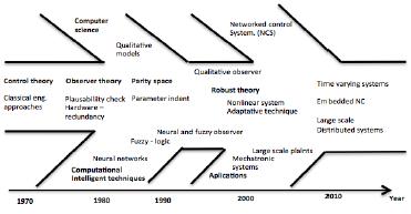
Another area is the applications, mainly driven by the urgent demands for highly reliable and safe control systems in the automotive industry, and the other areas are in the aerospace area, in robotics as well as in large scale, networked and distributed plants and processes. In the first decade of the short history of the model-based FDI technique, various methods were developed. During that time the framework of the model-based FDI technique had been established step by step. In his celebrated survey paper in Automatica 1990, Frank [41] summarized the major results achieved in the first fifteen years of the model-based FDI technique, clearly sketched its framework and classified the studies on model-based fault diagnosis into three methods too: ones are the observer-based methods, another are the parity space methods and the other parameter identification based methods.

In the early 90's, great efforts have been made to establish relationships between the observer and parity relation based methods. Several authors from different research groups, in parallel and from different aspects, have proven that the parity space methods lead to certain types of observer structures and are therefore structurally equivalent to the obserer-based ones, even though the design procedures differ. From this viewpoint, it is reasonable to include the parity space methodology in the framework of the observer-based FDI technique. The interconnections between the observer and parity space based FDI residual generators and their useful application to the FDI system design and implementation. It is worth to point out that both observer-based and parity space methods only deal with residual generation problems. In the framework of the parameter identification based methods, fault decision is performed by an on-line parameter estimation, as sketched in the Figure 1.

3.1 Qualitative Graphic Model

As we saw in the previous sections, currently modern industries are growing which means its scale and complexity is increased. This type of systems has many areas of process, tools, equipment and elements that interact constantly making it even more complex these systems. The failure diagnosis in such complex systems compared to the classical method of fault detection is that for complex systems analysis of fault propagation throughout the system which could lead to a catastrophic failure condition is required involving plant safety [42].

Models directed graphs (SDG) is the group of qualitative graphical models to describe process variables and their cause-effect relationships in continuous systems, where the process variables are represented as nodes and their relationships through directed arcs. The SDG obtained from flow diagrams, mathematical models and empirical knowledge is an expression of high knowledge. The search for patterns in the propagation of faults in a directed graph helps greatly and find the root causes [42] [43]. The hierarchical description of large scale complex systems is based on the decomposition and approximate aggregation, where a simple SDG level model can be transformed into a hierarchical model which makes it easier in the understanding of a complex system. [44] [45] [46]

The SDG model could be classified into three levels in a pyramid structure, even if the system is very large more levels can be considered. The upper level is also called system where the first level is divided into several sub-systems, sub-systems that can behave as separate components or interconnecting components that can not be separated. In the middle level, each control system is related to a super node. The principal steps to construct a SDG are: 1) Know the squeme process, P&ID and equations. 2) Identify the material flow diagram from relationships between the components. 3) According to the process knowledge determine the key variables. 4) Construct the SDG skeleton. 5) From the entire SDG include another variables and arcs. 6) Simplify and verify the SDG. 7) Validate the SDG with process data, simulations or experiments [42] [47].

3.2. Causal Graph Generation

The causal graph represents a group of influences between variables Vi, ... Vn with a set of relations among themselves r(Vi, ... Vn). Causality appears naturally in the differential equations representing the evolution on the time of the variables analyzed. Formally:

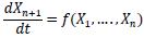
Where, it is accepted that the variable on the left side is causally dependent variables on the right side. Each influence is generally associated with a physical component, so if a variable influences another, the relationship of influence is associated with a component. The group of equations establishes the Structural Relation Model (SRM) which generated in five steps the Causal Model Structure (CMS) [46] [48]

4. Concepts of diagnosis

A system is said to be diagnosable if whatever the behavior of the system, we will be able to determine without ambiguity an unique diagnosis. The diagnosability of a system is generally computed from the model of the system. In applications using model-based diagnosis, such a model is already present and doesn't need to be built from scratch.

4.1 Observability

A system is fully observable if each state variables affecting any of the outputs. It is often necessary to obtain information on the state variables according to measurements of the inputs and outputs. If any state can not be seen from the measurements of the outputs it is said that the system is not completely observable or unobservable simply [49].

The fault diagnosis method based on discrete events can be classified into two groups depending on how the system is to diagnose: on-line diagnosis and off-line diagnostics [50]. The procedures for each of the cases are treated separately. In the off-line diagnostic system are available to perform tests on him, you can send scripts and get the evolutions of the system (equivalent to a verification of proper system operation). In the case of on-line systems, the fundamental methods for fault detection are based on Petri nets [51] [52].

4.2. Chronicle

A chronicle represent a group of signals associated to events of a system, and it defines a basic situation of a normal or abnormal change to be monitored. In addition, it is represented as a set of events and a set of temporal constraints between these events, associated to diagnosis messages depending on topological constraints [53]. The time then is one of the principal aspects of the analysis, because each time ocurrence event will be part to study and compared with a process model [54]. Chronicle models are sets of binary sequential relations with timed constraints between discrete event classes. A chronicle model represents an abstraction of the behavior of a dynamic system. The operationalisation of this behavioral knowledge with the DEVS formalism provides a formal semantic and allows the design of an ad hoc algorithm dedicated to recognizing subsequences of a given discrete event sequence that satisfies the sequential and the timed constraints of a given chronicle model [55].

The implementation is usually done through a control-monitor system capable of assessing the stage which is the process and takes appropriate decisions if you are in a fault situation. In many cases the method is based on Petri Nets or GRAFCET models and the control system is implemented in an industrial controller and the decision may be needed for example fuzzy an interpreter. The problems with these online systems are essentially two, which are presented below.

4.2.1. They must solve the problems of combinatorial explosion, for which you are defining different strategies, among which are the modular decomposition based methods, [51] [52] [56], however the main problem is found to establish a systematic method of decomposition that allows to application of complex systems.

4.2.2. The developed online systems currently work on systems whose evolution can be monitored completely, being able to implement the supervisor module externally-diagnostician [56], this scheme, which is the one that is working on some complex processes with slow changes, may behave inefficiently in systems with rapid change. To solve this problem have been chosen to perform the following modifications:

4.2.2.1. The diagnostic system is implemented in the control system (PLC). In this configuration, the control system is extended to be able to perform self-diagnosis. It would be an evolution of the traditional method is added diagnostic capabilities. In some cases, this identification is validated by an operator and sent to the centralized registration system breakdowns [1].

4.2.2.2. The monitoring and diagnostic system is implemented in a mixed solution (external equipment Assist. Controls). Diagnostic tool and guidance will be implemented on an external device, e.g. a computer program, which runs on a PC connected to the control system. This team will have direct access to the system, so that the diagnostic system and guided all the information requested is necessary for the diagnosis, monitoring and guiding.

4.3. Timed Diagnosability

The standard definition of diagnosability of DES according to the problem is to detect the occurrence of unobservable fault events using "inference" based on models from observed event sequences (chronicles) [57]. One of the major drawbacks to achieve fault-tolerant supervision of discrete event systems is considered from the point of view of safe and timely diagnosis of unobservable faults. Thus the moon diagnosability is presented as new security feature. If the system is diagnosable reconfiguration actions could be forced failure detection prior to execution of unsafe behavior, thus achieving the goal of fault tolerant supervision. Detecting "before" the unsafe behavior, involves time as a key variable in the process, hence the term "Timed diagnosability". The occurrence of a fault is diagnosed by analyzing the flow of observations and matching this flow with a set of available chronicles [20].

5. Application of chronicles

In complex dynamic systems the data comes out from sensors and this information must increase continuously. Diagnosis of the system involves identify the elements failure using observations derived from the streaming data. The supervision of these dynamic requires a monitoring system to identify abnormal situations in less amount of time. Typical monitoring systems consist of the follow three modules: 1) Detection module, 2) Diagnostic module and 3) Decision module [58], as can be see in the Figure 2.

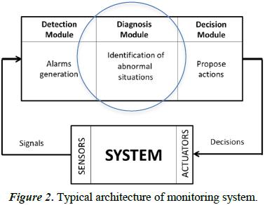
The detection module continuously monitors signals provide by the sensors and decides if the systems behavior is normal or the signal values activate some alarm. The diagnosis module is responsible for analyzing alarms in order to identify abnormal situations and the diagnosis of a corresponding failure and that is where we propose to apply an effective methodology. The diagnosis can be performed by recognition of chronicles because each failure must be associated with a chronicle which corresponds to some abnormal situation. The expert systems based their reasoning on rules, reducing in importance time information but, when the safety in a process could be affected the time is an important aspect to analyze particularly when alarms are activated and the operator need recognize it. The recognition of chronicles is based on diagrams of evolution in which time is fundamental. Chronicles provide a framework for modeling dynamic system and this tool has been proposed by Dousson et. al. since 1993 [59].

A chronicle is a partial order of events with time constraints and it associates with the occurrence of a fault. The situation recognition system performs recognition of instances of occurring situations, as they are developing and it generates events and actions that must be detected. The alarms in systems are events that require actions by the operator and when the number of alarm increase it need be processed for reducing the quantity and allowing an effective response of the operator [8] [59] [60] [61] [58].

A chronicle is composed of the following three parts:

-A set of predicates
-A set of temporal constraints which relate these predicates
-A set of actions to be taken when the chronicle is recognized

Then, a chronicle representation relies on a propositional reified logic formalism in which the environment is described through domain attributes and messages where their temporal qualifications are formed using different types of predicates. Then, the chronicles are a temporal pattern that represents the possible evolution of the system where a set of events are related by time constraints.

5.1. Time Representation

Relies on the time points algebra where time is considered as a linearly ordered discrete set of instants. A time interval I is expressed as pair I=(t₁, t₂) corresponding to the lower and upper bound on the temporal distance between two time points t₁ and t₂. Time is considered as a linearly ordered discrete set of signals where we can handle the usual symbolic constraints of the time point algebra as well as numerical constraints. Then, I(e₁→e₂) = [I^-,I⁺] it express the time distance between the events.

5.2. Reifying Predicates

Reifying Predicates are used to temporally qualify the set of domain attributes. In the literature we can find the next predicates used in a chronicle.

5.3. Basic Chronicle Patterns

The domain attribute P must keep the value v over the interval [t₁,t₂];

Message P occurs at t;

If any change in P occurs between t1 and t2 the chronicle can not be recognized;

The event a must keep the value over the interval t₁, t₂;

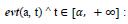an event a occurs after α time units;

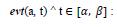an event a occurs between α and β time units;

an event a occurs without any prior event b;

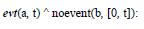
no event a occurs between α and β time units;

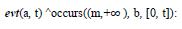an event a occurs after at least m events b;

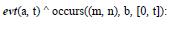an event a occurs after at least m and at most n events b.

An event has no duration. Events denote a change of the value of a domain attribute.

5.4. Domain Attribute

In the reified logic formalism, the environment is described through domain attributes. Domain attributes are the atemporal propositions of the modeled environment. The domain attribute is a couple P(α₁,...α_n):ν where P is the attribute name, α₁,...α_n its arguments and v its value. For example:

hold (P: v, (t₁, t₂)) The domain attribute P must keep the value v over the interval t₁, t₂

6. Automated translation of chronicles

The basic system should behave as a timed model M = (E, T) with a set of events E as of trajectories of the system (i.e. the system language) and a set of constraints of time T between the occurrence date events. Among the events produced by the system, some of which are observable as well as the date of occurrence of observable timed model (EOB, TOBS) so that M can be characterized by projection [20].

A chronicle is a set of observable events with some time constraints. A good account is used to describe a situation based on their observable effects [62]. In a diagnostic approach based on chronicle, each abnormal situation (ie, a failure) is usually associated with a number of chronic, chronic recognizes each sub-part of the corresponding error associated with this sequence. That is when a process is being presented unusual actions according to the model obtained are projected to set corresponds to failure. A positive aspect of these approaches is their high efficiency due to the fault indication based on expert systems. The downside is usually the difficulty of acquiring and chronic database update these systems.

Chronicle recognition can be performed as follows, given a flow of observable events, a system for recognition of chronic is responsible for checking on the progress if the flow coincides with some of the chronic basis. It is said that the model is recognized if the flow event case contains an instance of each event in the chronic model meet these instances time constraints defined in the chronic model. A chronicle is a partial order of events with time constraints and is associated with the occurrence of a fault. It is a model c is a pair (S, T) where S is a set of observable events and T a set of constraints between their occurrence dates.

More formally: A chronic model c = (S, T) is recognized in a sequence σ observable event instances if and only if:

- there exists, for all event (ei, ti) ∈ S = {(e1, t1), . . ., (en, tn)}, an event instance (ei, ti|) in σ and

- the constraint system {t1 = t₁|, ..., tn = tn } ∪ T is satisfiable.

The set of trajectories of the system leading to the recognition of the chronicle c is called the recognition language L(c). Each abnormal situation or fault f that is the observable behavior of the system when the fault occurs. A chronicle model c(f) is associated to a fault f when its observable recognition language Cf is a subset of the fault signature Cf C Sig(f).

6.1. General Principle of the Analysis

Two chronicles are exclusive if they cannot be recognized with the same flow of event instances. It has been shown that the proposed exclusiveness analysis can be performed relying on two kinds of inputs.

6.1.1. Translation

The objective of this step is to translate each chronicle model into Labeled Time Petri Net with Priorities (LTPNPr). Time Petri Net with Priorities (TPNPr) is an extension of TPN in which a priority relation on transitions is defined [63].

6.1.2. Product

The exclusiveness test aims to check that the chronicles cannot be recognized by a common trajectory of events.

6.1.3. Exclusiveness test

The exclusiveness analysis must deal with an important number of trajectories that may induce the chronicle recognition what is called chronicle instances.

The objective of the product of the Petri Nets is to represent in a single model the common behaviors of two chronicles but also the independent behaviors of each chronicle, a specific product for LTPNPrs obtained by adding transitions labeled with synchronized events (common events) and by adding priorities relations involving these new transitions if necessary.The transition from which the arc comes out has a higher priority than the transition in which the arc comes in. Thus, in case of simultaneous activation, the transition with a higher priority is triggered.

7. Proposed model analisis.

Lets go to construct a special fault detection model using the causal graph and the chronicles as combined methods for an Alarm management preliminar methodology. First, in a singular process structure we will construct his causal graph and after we will determinate the chronicles for normal behavior of the startup procedure in this process. The process is composed by a tank (TK), two valves (V1 and V2), a pump (Pu), a level sensor (LT), a pressure sensor (PT) and a flow sensor (FT) see Figure 3.

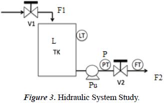
This process is a pressuring system which is composed by the follow ecuations:

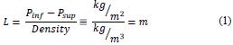
The level into the tank is determinated by the method HTG (Hidrostatic Tank Gauging) using the hidrostatic pressure and the liquid temperature into the tank. Then, the level sensor is determine by a differential pressure sensor that indicate the difference between the pressure on the tank base (P_inf) and the superior pressure of the tank (P_sup) divided by the density of the liquid. The density is calculated by the differencial pressure between the pressure on the button and the pressure in the middle with a fixed distance between both (h). Then, the level is determine in the equation e₁:

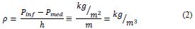
The density is determine in the equation e₂:

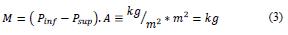
The mass of the liquid is determine in the ecuation e₃, in this equation A is the area of the tank.

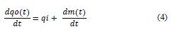
The relationship between the input (qi) and output (qo) mass flow in the tank is related with the change of the mass or weight into the tank. This reltationship is determine in the differential ecuation e₄:

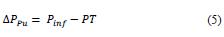
The differential pressure in the pump Pu is determine in the ecuation e₅:

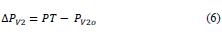
The differential pressure in the valve V2 is determine in the ecuation e₆:

7.1. Steps for Generating the Causal Graph

Below are shown the five key steps in the generation of the Causal Model Structure (CMS)

7.1.1. First step

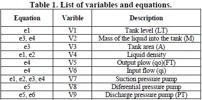
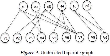
In the Graph Theory, a bipartite Graph is a Graph G=(N,E) whose vertices can be separated into two disjoint sets U and V so that the edges only can connect vertices of a set with other vertices, Bipartite graphs are often represented graphically by two columns (or rows) of vertices and edges joining vertices of different columns (or rows). Then, the first sept is to generate a preview bipartite Graph G=(V ∪E,A) where V is the set of variables, E is the set of equations and A is the arcs or relationships between equations with variables, these relationships have no direction. For our case, the list of variables with the ecuations is exposed in the Table 1.

Creating the Graph bipartite as can see in the Figure 4:

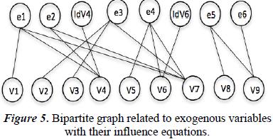
7.1.2. Second step

In this step we identify the exogenous variables, therefore an influence equation (Id) will be associated to each exogenous variable. In this case, the exogenous variables are the tank inflow (IdV6) and the liquid density (IdV4). Then, this is the Bipartite graph with the influence equations in the exogenous variables.

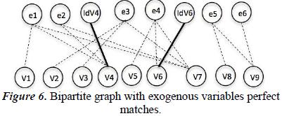
7.1.3. Third step

In this step we need to identify which equations involve just one variable, in this case, the exogenous variables; look at Figure 6.

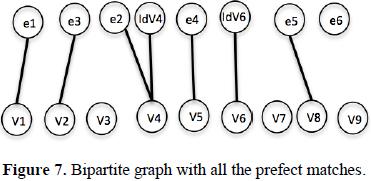
7.1.4. Fourth step

We need to identify the perfect matching. It is, only when the equation relates one variable, for example, the variable V1 with e1, e3 with V2 and the others variables V4, V5, V7 and V8, according with the Figute 7.

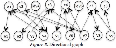
7.1.5. Fifth step

The directional graph is derived from the perfect links. E to V are routed in this direction and in other cases is routed from V to E. See Figure 8.

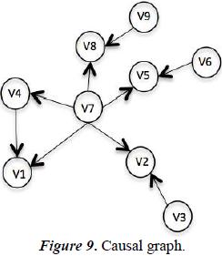
7.2. Generating Causal Graph

From the directional graph the causal graph is built G_c=(V,I) in the equation V is the Variables and I as the directional relationships. In this graph don't appear the equations nodes. Look at the Figure 9.

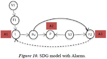
7.3. Suppression of Variables

We can remove unmeasured variables or variables that do not influence significantly on other variables. In this case we will remove the variable V3 because the area Tank does not change. We remove the variable V2 because we do not measure the weight (See the Figure 10).

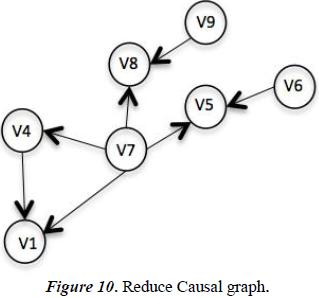
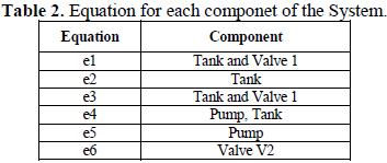
The causal graph could be constructed using the tool "Causalito" [48, 46]. For do that, we need construct a matix formed by the components and the variables. The components are related with the ecuations as it is show in the following table (Table 2):

The matrix that relate the components with the variables is give by Table 3:

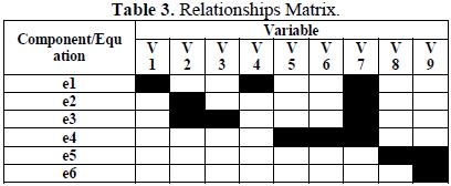
The SDG model for this process is conventional by the representation of the process variables as graph nodes and representing causal relations as directed arcs. An arc from a node X to node Y implies that the deviation of X may cause an deviation of Y. Figure 10.

7.4. Chronicle Example

One of the most important steps for fault detection is to determine the sequence of events that can be carried to a failure. Each situation model is a set of event patterns and temporal constraints between them; then a situation model may also specify events to be generated and actions to be triggered as a result of the situation occurrence. In an industrial process, especially on the petrochemical sector the alarm management is an important aspect.

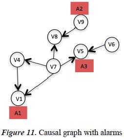
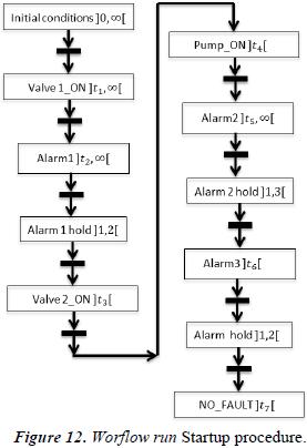
For the startup procedure in the example process we will construct the next chronicle than describe the normal behivor, where: ValveV1_ON, ValveV2_ON, PumpPu_ON, Alarm_1, Alarm_2, and Alarm_3 are observable events in the system. The Alarm_1 is the alarm of high level in the tank, Alarm 2: outlet high pressure and Alarm 3: outlet high flow. Then, in the startup procedure for this part of the process the six steps are: First, check the initial conditions like valves off, pump off, tank empty. Second, turn ON the Valve 1 after t₁ time units. Third, wait to the liquid full the tank after t₂ time units, this Alarm_1 must be activate between 1 and 2 time units. Fourth, turn ON the valve 2 to t₃ time units. Fifth, turn ON the pump to t₄ time units. Sixth, wait to the pressure outlet will be in high

(Alarm_2) after t5 time units and it must hold between 1 and 3 time units. Seventh, wait to the maximun flow will be reached, the Alarm_3 activate to t6 time units and it must hold between 1 and 2 time units. On the Causal Graph the alarms are located as show the Figure 11.

Diagnosis depends on an event-based method for the monitoring approach. A workflow describes then a partial order of events and a workflow run is a arrangement of event instances: (e1, t1) . . . (en, tn) where (e1, t1) could be the first event instance of the run [61] [64]. From startup procedure and causal graph we construct the workflow run for describe after the chronicle, as can see in the Figure 12.

Chronicle:

evt(InitialConditions)
evt(ValveV1_ON, (t₁, +t₁, +∞))
evt(Alarm_1, (t₂, +t₁, +∞))
hold (Alarm1, (1,2))
evt(ValveV2_ON, t₃ )
evt(PumpPu_ON, t₄ )
evt(Alarm_2, t₅)
hold (Alarm2, (1,3))
evt(Alarm3, t₆ )
hold (Alarm3, (1,2))
t₁<t₂<t₃<t₄<t₅ <t₆ <t₇

When recognized

emit event ( NO_FAULT, t₇)

Pattern combination:

C: evt(InitialConditions) ^ evt(ValveV1_ON, (t₁, +∞))^ evt(Alarm_1, (t₂, +∞)) ^ hold (Alarm1, (1,2)) ^ evt(ValveV2_ON, t₃ ) ^ evt(PumpPu_ON, t₄ ) ^ evt(Alarm_2, t₅) ^ hold (Alarm2, (1,3)) ^ evt(Alarm3, t₆ ) ^ hold (Alarm3, (1,2)) ^ t₁<t₂<t₃<t₄<t₅ <t₆ <t₇

A Failure Mode Analysis (FMA) is required to determine all the possible chronicles that carried the system to an inminent failure. The process for managing Risk is followed basically into four steps: Information on the process. Identity hazards, Evaluate risks and Specific risk reduction measures. After obtaining all the chronicles necessary a pattern reconigtion with a search motor which in real time recognize the "good" and "bad" chronicles [47] [65].

8. Conclusions

A preliminar basic method for an Alarm management with fault diagnostic was present using the Causal graph and the Chronicles as the fault diagnostic techniques. When the process is new the analisys of a chronicle and determinate the unobservable events and fails could be problematic. The determination of some base chronicle requires of hystoric data and experience with the process dinamic.

The use of LTPNPrs to recognize the chronicles could be remplaced for a GRAFCET model to check signals of alarms in a process in a next job. Another possible continuation of this analysis would be the study of the design a method, strategy or approach for design and structure a alarm management on starting process for fault diagnostic.

The evolution of the model shows how the process progresses and we can have information to determinate if if the actual process is evolving correctly or not.

The next analysis could be the use of Chroniques apply to the model for structure a new model that can determinate the good chroniques of the system comparing with the operation on real time of the process.

References

[1] R. Brennan, «Toward real-time distributed intelligent control: A survey of research themes and applications,» IEEE Trans. Syst., Man, Cybern. C, Appl. Rev, vol. 37, nº 5, pp. 744-765, Sep. 2007.         [ Links ]

[2] M. Khalgui, O. Mosbahi, Z. Li y H. Hanisch, «Reconfiguration of distributed embedded-control systems,» IEEE/ASME Trans. Mechatronics, vol. 16, nº 4, pp. 684-694, Aug. 2011.         [ Links ]

[3] M. G. Mehrabi, A. G. Ulsoy y Y. Kore, «Reconfigurable manufacturing systems: Key to future manufacturing,» Journal of Intelligent Manufacturing, 2000.         [ Links ]

[4] H. Pentti y H. Atte, «Failure mode and effects analysis of software-based automation systems,» VTT Ind. Systems STUKYTOTR, vol. 190, nº 09, p. 37, 2002.         [ Links ]

[5] I. Yélamos Ruiz, A global approach for supporting operators decision-making dealing with plant abnormal events, Barcelona: Universidad Politecnica de Cataluña, 2008.         [ Links ]

[6] T. Stauffer, N. Sands y D. Dunn, «ALARM MANAGEMENT AND ISA-18 - A JOURNEY, NOT A DESTINATION,» de Texas A&M Instrumentation Symposium , 2010.         [ Links ]

[7] V. Venkatasubramanian y et. al., «A review of process fault detection and diagnosis. Part I: Quantitative model-based methods,» Computers and Chemical Engineering, 2003.         [ Links ]

[8] ISA-TR84.00.02, «Safety Instrumented Functions (SIF) - Safety Integrity Level (SIL)»         [ Links ].

[9] E. Habibi y B. Hollifield, «Alarm systems greatly affect offshore facilities amid high oil prices,» World Oil, pp. 101-105, September 2006.         [ Links ]

[10] E. García, C. Agudelo, F. Morant y E. Quiles, «Secuencias de alarmas para detección y diagnóstico de fallos,» de 3er Congreso internacional de ingeniería mecatrónica, Valencia, Spain, 2012.         [ Links ]

[11] L. Amendola, «Aplicación de la Confiabilidad en la Gestión de Proyectos en Paradas de Plantas Químicas,» de Papers VI Internacional Congreso on Project Engineering, AEIPRO, Barcelona, Spain, Octubre, 2002.         [ Links ]

[12] L. Amendola, «Project Optimization of Plant Stoppages,» USA, 2002.         [ Links ]

[13] P. Bonnal, D. Gourc y G. Lacoste, «The Life Cycle of Technical Projects,» Papers Project Management Institute, vol. 33, nº 1, pp. 12-19, March 2002.         [ Links ]

[14] Delta Catalytic Industrial Services, Turn around Management Program, Process Effectiveness Assessment Workbook, 2000.         [ Links ]

[15] H. Kerzner, Applied Project Management Best Practices on Implementation, New York: John Wiley & Sons, Inc., 2000.         [ Links ]

[16] H. Levine, Practical Project Management, New York: John Wiley & Sons, Inc., 2002.         [ Links ]

[17] PMI Standards Committee, A guide to the Project Management Body of Knowledge, 2000.         [ Links ]

[18] J. Voivedich y E. Ben, Risky Business Developing a Standardized WBS to Mitigate Risk on Refinery, Turnarounds, 1998.         [ Links ]

[19] S. Adhikari y C. Bayley, Reliability Analysis: A Review and Critique, Manchester Business School, 2010.         [ Links ]

[20] S. Cauvin, M. Cordier, C. Dousson, P. Laborie, F. Lévy, J. Montmain, M. Porcheron, I. Servet y L. Travé-Massuyès, «Monitoring and alarm interpretation in industrial environments.,» Journal: AI Communications, vol. 11, nº 3-4, 1998.         [ Links ]

[21] T. Strasser, «AUTONOMUS APPLICATION RECOVERY IN DISTRIBUTED INTELLIGENT AUTOMATION AND CONTROL SYSTEMS WITHIN,» 2012.         [ Links ]

[22] J. von Neuman, «Probabilistic Logics and the Synthesis of Reliable Organisms from Unreliable Components,» de Automata Studies, Princenton, NJ, Princenton University, 1956, pp. 43-98.         [ Links ]

[23] E. F. Moore y C. E. Shannon, «Reliable Circuits Using Less Reliable Relays,» pp. 191-208, 1956.         [ Links ]

[24] W. H. Pierce, Failure tolerant computer design, New York: Academic Press, 1965.         [ Links ]

[25] A. Avizienis, «Design of fault-tolerant computers,» Proc. 1967 Fall Joint Computer Conf, vol. 31, pp. 733-743, 1967.         [ Links ]

[26] W. Elmendorf, «Fault-tolerant programming,» de Proc. 2nd IEEE Int, Symp. on Fault-Tolerant Computing, Newton, Massachusetts, June 1972.         [ Links ]

[27] B. Randell, «System Structure for Software Fault Tolerance,» IEEE Trans. on Software Engineering, Vols. 1 de 2SE-1, nº 2, pp. 220-232, 1975.         [ Links ]

[28] A. Avizienis y L. Chen, «On the implementation of N-version programming for software fault tolerance during execution,» Proc. IEEE COMPSAC, vol. 77, pp. 149-155, Nov. 1977.         [ Links ]

[29] J. Laprie y A. Costes, «Dependability: A Unifying Concept for Reliability Computing,» de Proceedings of the IEEE Symposium on Fault Tolerant Computing, 1982.         [ Links ]

[30] B. Randell y J. Dobson, «Reliability and Security Issues in Distributed Computing Systems,» de 5th IEEE International Symposium on Reliability in Distributed Software and Database Systems, Los Angeles, CA, USA, 1986.         [ Links ]

[31] M. K. Joseph y Avizienis, «A Fault-Tolerant Approach to Computer Viruses,» de In Proc. 1988 Symposium on Security and Privacy, 1988.         [ Links ]

[32] J. Fray, Y. Deswarte y D. Powell, «Intrusion tolerance using fine-grain fragmentation-scattering,» de Proc. 1986 IEEE Symp. on Security and Privacy, Oakland, April 1986.         [ Links ]

[33] A. Avizienis y Y. He, «Microprocessor entomology: a taxonomy of design faults in COTS microprocessors,» Dependable Computing for Critical Applications, pp. 3-23, 1999.         [ Links ]

[34] A. Avizienis y J. Kelly, «Fault tolerance by design diversity: concepts and experiments,» Computer, vol. 17, nº 8, pp. 67-80, Aug. 1984.         [ Links ]

[35] W. Bouricius, W. Carter y P. Schneider, «Reliability modeling techniques for self-repairing computer systems,» de Proceedings of 24th National Conference of ACM, 1969.         [ Links ]

[36] P. Jackson, Introduction to Expert Systems, Addison-Wesley, 1986.         [ Links ]

[37] A. Mei Chen, H.-m. Lu y R. Hecht-Nielsen, «On the Geometry of Feedforward Neural Network Error Surfaces,» Neural Computation, vol. 5, nº 6, pp. 910-927, 1993.         [ Links ]

[38] G. Menkhaus y B. Andrich, «Metric suite for directing the failure mode analysis of embedded software systems,» Inf. Syst. J, pp. 226-273, 2005.         [ Links ]

[39] R. Brennan, M. Fletcher y D. Norrie, «An agent-based approach to reconfiguration of real-time distributed control systems,» IEEE Trans. Robot. Autom, vol. 18, nº 4, pp. 444-451, 2002.         [ Links ]

[40] S. X. Ding, «Model-based Fault Diagnosis Techniques Design Schemes, Algorithms, and Tools,» 2008.         [ Links ]

[41] F. P. Lees, «Loss Prevention in the Process Industries,» 1995.         [ Links ]

[42] F. Yang, D. Xiao y S. L. Shah, «Qualitative Fault Detection and Hazard Analysis Based on Signed Directed Graphs for Large-Scale Complex Systems,» 2010.         [ Links ]

[43] F. Yang y D. Xiao, «Approach to modeling of qualitative SDG model in large-scale complex systems,» Control Intrum. Chem. Ind., vol. 32, nº 5, pp. 8-11, 2005.         [ Links ]

[44] S. Gentil y J. Montmain, «Hirarchical representation of complex systems for supporting human decision making,» Advanced Engineering Informatics, vol. 18, nº 3, pp. 143-159, 2004.         [ Links ]

[45] H. A. Preisig, «Constructing, modifying and maintaining consisten process models,» de FOCAPD, Colorado, June 7-12, 2009.         [ Links ]

[46] B. Celse, S. Cauvin, B. Heim, S. Gentil y L. Travé-Massuyés, «Model Based Diagnostic Module for a FCC Pilot Plant.,» Oil & Gas Science and Technology - Rev. IFP, vol. 60, nº 4, pp. 661-676, 2005.         [ Links ]

[47] V. Venkatasubramanian, J. Zhao y S. Viswanathan, «Intelligent systems for HAZOP analysis of complex process plants,» Purdue, 2000.         [ Links ]

[48] L. Trave-Massuyes y R. Pons, «Causal ordering for multiple mode systems. Laboratoire d Analyse et d Architecture des Systemes du CNRS,» 1995.         [ Links ]

[49] B. C. Kuo, Automatic Control Systems.         [ Links ]

[50] B. Bavishi y E. Chong, «Automated fault diagnosis using a discrete event systems framework,» de Proc. 9th IEEE Int. SYMP, 1994.         [ Links ]

[51] Cicslak, Desclaux, Fawaz y Variya, «Supervisory control of discrete event processes with partial observations,» IEEE Trans. Automat. Contr, vol. 33, nº 3, pp. 249-260, Mar 1988.         [ Links ]

[52] R. Ferreiro y B. Rodriguez, «Process control failure diagnostic fuzzy expert system,» de International Conference on Fault diagnosis, Tolouse, 1993.         [ Links ]

[53] J. Taisne y Autom. & Inf. Syst., AREVA T&D, «Massy Intelligent Alarm Processor based on Chronicle Recognition for Transmission and Distribution System,» 2006.         [ Links ]

[54] J. Taisne y A. t&d, «Intelligent Larm process for DMS based on "Chronicle" concept,» de 19 th International Conference on Electricity Distribution, France, 2007.         [ Links ]

[55] M. Le Goc, P. Bouch y N. Giambiasi, DEVS, a formalism to operationnalize chronicle models in the ELP laboratory, 2006.         [ Links ]

[56] E. Garcia Moreno, «Modular Fault diagnosis based on discrete event systems for a mixer chemical process,» de Congreso ETFA-99, Barcelona, España, 1999.         [ Links ]

[57] A. Paolia y S. Lafortune, «Safe diagnosability for fault-tolerant supervision of discrete-event systems,» Automatica, vol. 41, nº 8, pp. 1335-1347, August 2005.         [ Links ]

[58] R. D. Quiniou y T. D. Guyet, «Concept change detection and model adaptation for chronicle recognition based diagnosis,» Rennes, France, 2003.         [ Links ]

[59] C. Dousson, P. Gaborit y M. Ghallab, «Situation recognition: representation and algorithms,» de IJCAI: International Joint Conference on Artificial Intelligence, Chambéry, France., 1993.         [ Links ]

[60] M. Cordier y C. Dousson, «Alarm driven monitoring based on chronicles,» de 4th Sumposium on Fault Detection Supervision and Safety for Technical Processes (SafeProcess), Budapest, Hungary, 2000.         [ Links ]

[61] B. Morin y H. Debar, «Correlation of Intrusion Symptoms : an Application of Chronicles,» Caen, France, 2002.         [ Links ]

[62] H. Gougam, A. Subias y Y. Pencolé, «Timed Diagnosability Analysis based on Chronicles,» 2012.         [ Links ]

[63] B. Berthomieu, F. Peres y F. Vernadat, «Bridging the gap between Timed Automata and Bounded Time Petri Nets.,» FORMATS, LNCS, vol. 4202, pp. 82-97, 2006.         [ Links ]

[64] S. A. Pencole Y., «A Chronicle-based Diagnosability Approach for Discrete Timed-event Systems: Application to Web-Services.,» Journal of Universal Computer Science, vol. 15, nº 17, pp. 3246-3272, 2009.         [ Links ]

[65] R. Asok, «Symbolic dynamic analysis of complex systems for anomaly detection»         [ Links ].