DOI: http://dx.doi.org/10.18180/tecciencia.2014.17.8

Design of a sound pressure level acquisition and analysis system

Diseño de un Sistema de adquisición y análisis de nivel a presión sonora

Julian F. Casas¹, Paula T. Noreña², Luís F. Hermida³

¹ Universidad de San buenaventura, Bogotá, Colombia, jfcasas@academia.usbbog.edu.co
² Universidad de San buenaventura, Bogotá, Colombia, pnorena@usbbog.edu.co
³ Universidad de San buenaventura, Bogotá, Colombia, lhermida@usbbog.edu.co

How to cite: Casas, J.F. et al., Design of a sound pressure level acquisition and analysis system, TECCIENCIA, Vol. 9 No. 17, 61-66, 2014, DOI: http://dx.doi.org/10.18180/tecciencia.2014.17.8

Received: 16/08/2014 Accepted: 20/09/2014 Published: 30/12/2014

Abstract

This study focuses on the development of an analysis and acquisition software for sound pressure levels in industrial areas, designed and optimized to comply with the requirements of international standard ISO 7731 ("Danger Signals for Public and Work Areas" [1]) by performing a study of octave band equivalent sound pressure levels from 125 Hz to 8 KHz. The software and algorithms proposed are linked with other codes to perform a complete analysis for the above standard. The software we outline focuses on the capture process for subsequent analysis and can be applied not only for application with ISO 7731 [1] but also for the acquisition of equivalent sound pressure levels in any field of study. However, one needs to bear mind that the hardware used in data acquisition must comply with quality requirements and may directly cause systematic errors in the results. The main achievement of this study is the use of acoustic theory (as taught in university) to develop high-quality data acquisition systems that can be applied in academic projects and research projects, thus removing an obstacle in scientific and engineering development.

Keywords: Alarm, Background Noise, ISO 7731, Software Development, Sound Pressure Level (SPL).

Resumen

El presente trabajo se enfoca en la realización de un software de captura y análisis de datos de nivel de presión sonora en áreas industriales, diseñado para aplicar la normativa internacional ISO 7731 ("Danger Signals for Public and Work Areas") [1], realizando un estudio de nivel de presión sonora equivalente por bandas de octava desde los 125 Hz hasta los 8 KHz. Junto con el software y algoritmos propuestos se encuentran enlazados otros códigos para realizar un análisis completo de la normativa citada anteriormente. El software explicado a continuación se enfoca en la sección de captura para su posterior análisis y puede ser aplicado no solo para fines de análisis de la normativa ISO 7731 [1] sino como obtención de niveles de presión sonora equivalentes en cualquier campo, pero se debe tener en cuenta que el equipo utilizado para su captura influye directamente a los resultados obtenidos. El principal desarrollo del presente proyecto es la utilización de la teoría acústica impartida en la academia para desarrollar sistemas de captura de alta calidad que puedan ser aplicados en estudios académicos y desarrollos de proyectos de investigación, eliminando de esta manera un obstáculo para el desarrollo científico e ingenieril.

Palabras claves: Alarma, Desarrollo de Software, ISO 7731, Nivel de Presión Sonora (NPS), Ruido de Fondo.

1. Introduction

The use of sound pressure levels (SPLs) grouped by octave-band and 1/3 octave-band is one of the main tools for analyzing a noise field with a specific signal of interest, including traffic noise, ambient noise, alarm signal transmission analysis, the acoustic parameters of a concert hall, and the levels permitted under international standards. It is even used in fields of knowledge as diverse as health, ecology, civil engineering, and economics [2]. It is for this reason that programming software which specializes exclusively in the acquisition of such data is of great assistance to a sound engineer or acoustic engineer that can use the results for programming or analyze the results for a specific study.

One method of obtaining these results is through the use of sound level meters (SLMs) that meet the specific international standards necessary for acquisition. Yet, it must be emphasized that these systems entail a high cost and are not affordable for one demographic interested in obtaining and analyzing such results — students who require a system of acquisition and analysis in their studies and need conclusive, effective, and quick learning.

The software in this study, created in the MatLab platform, is focused on obtaining SPL results per octave-band and obtaining an equivalent SPL for the entire capture. Results are displayed under the frequency weightings flat, A-weighting, and C-weighting, in order to analyze any output that emerges for different applications of analysis in the field of acoustics.

The software is called Análisis de Alarma 2.0 (Alarm Analysis 2.0) since it was specifically designed for the analysis of industry alarm systems according to the standard ISO 7731, Danger Signals for Public and Work Areas [1]. Thus, only data between the 125 Hz and 8000 Hz bands are analyzed. Two sound recordings must be made, for both background noise and for the capture of the industry alarm signal.

It must be clarified that the algorithms used for the analysis can also be used for all required bandwidth. This is in case the study of specific spectrums or ranges of frequencies required by another standard is desired. Additionally, the hardware utilized, such as the transducer and the data capture card, must be of sufficient quality so as to validate the results obtained by the software.

2. Equipment used

To create this acquisition and analysis software, one must use (as explained above) the equipment necessary for achieving the acquisition with the lowest possible introduction of noise from other sources (whether electronic or system failure). With this objective in mind, the following equipment was used:

• Data acquisition card: RME FireFace 400
• Input transducer: Earthworks M30
• Alarm transmission (Pink Noise): Dodecaedro 01dB
• Sound level meter (SLM): Svan
• MatLab 2013
• Svan Pistonphone

All of the above equipment meets the necessary quality requirements for this research project. Since the effectiveness of the designed software must be verified with a tool dedicated to such a task, we decided to use the Svan SLM to compare the results of equivalent levels between the studied bandwidths and an omnidirectional source of pink noise. This establishes behavioral relationships not only in the alarm transmission frequencies according to the standard, but also in all frequency bands [3].

3. Algorithms used

The proposed system must be capable of obtaining equivalent SPLs from both background noise and industry alarm signals in order to meet the data analysis requirements of the ISO 7731 standard [1]. Therefore, the algorithms used throughout the various sections of the software must be studied in order to understand how results were obtained and to characterize the data flow throughout the program.

3.1. Calibration Section

For the calibration section of the software, it is necessary to determine whether to proceed to work with one or two independent channels. These must go through the same 5-second calibration process, with additional time to process the respective calculations [4]

There are two SPL options for the calibration: the first is by recording the 1KHz transmission at 94 dB SPL and the second is recording the 1KHz transmission at 114 dB SPL. The user can choose either option. Selection criteria is based on the background noise found at the exact moment that the calibration of the M30 transducers is executed. If background noise is considerable, it is preferable to use a high level of calibration (in this case 114 dB SPL) to avoid potential errors deriving from the undesired increase in pascals due to incidental noise [5].

After the acquisition by means of simple codes in MatLab, a window function must be applied. In this case the Hamming algorithm was chosen, since it preserves a great deal of the original signal and rejects errors at the beginning and end of the recording which can produce decisive errors in the subsequent Fourier analysis. [2]

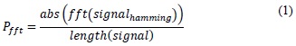
After applying the preceding algorithm to the signal, a quick Fourier transform is performed to obtain signal data in the frequency domain. As is well-known, the Fourier transform¹ maps the real and imaginary parts of the amplitude of a signal. It is therefore necessary to obtain only the real parts and duplicate the energy displayed to obtain the values of interest for our program [6].

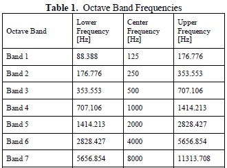
After obtaining the energy representative of the signal in the frequency domain, it is necessary to study the amount of energy in the 1KHz² octave band. First, we must determine what the frequency limits of the studied band are. We obtained a lower frequency limit of 707.1 Hz and an upper limit of 1414.2 Hz. With these frequencies determined, the process to obtain the value of the total amplitude found in this band (corresponding to 94db SPL on the pistonphone) was carried out by summing the amplitudes of the samples within this frequency range in the variable Pfft. Now, considering that the SPLs cannot have linear relationships with the data obtained in the displayed algorithms, one must first calculate the logarithmic relationships of the energy within octave bands. Afterwards, a conversion to absolute pascals may be implemented in order to linearize the model.

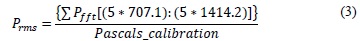
Once the relationship in expression No. 3 is obtained, the calibration section is finished. It needs to be mentioned that the process of system calibration should always be performed before obtaining representative results, in order to comply with international standards of sound pressure data measuring [7].

3.2. Recording of Signals of Interest

In this section of the software, the recording of only two types of signals of interest for ISO standard 7731 is performed — the SPLs of the background noise and of the alarm. For this, the user must enter the length of time in seconds in which he wants to collect data for subsequent analysis. For the ease of use of the user interface, two sections with colors have been activated which allow the user to know if the data collection process has finished (green) or is still in process (red). If the software is taking more than 10% of the entered length of time in seconds for the recording, this suggests that an error has occurred and restarting the program and taking the measurements again is recommended.

3.3. Analysis of the Recordings

This section is the cornerstone of the software and the place where the most errors occurred in the performed tests. It therefore must be studied in depth to understand the data flow throughout the program in order to obtain equivalent SPL results in different weightings.

The first step in carrying out the analysis on the recording of background noise and alarm signal is to divide the entire recording into sections of equal quantities of samples. This is done in order to study, in as detailed a fashion as possible, the total obtained data recording. In accordance with international standards, this section corresponds to the type of time analysis or time weighting that is used in data logging for different applications, found under the names Slow (1 second), Fast (125 milliseconds), and Impulsive (35 milliseconds). For this application, the Fast weighting is used. In other words, for a total recording of 5 seconds, the program would divide the total time into 40 micro-recordings which would then be analyzed individually, taking into account expressions and algorithms 1, 2, and 3 of the calibration section [8].

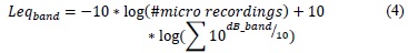
After individually analyzing the micro-recordings by octave band³ and making a pressure comparison in pascals with the last values obtained in the calibration section, the SPL data is stored in vectors (both the data and the micro-recordings). These will later be used to obtain the equivalent SPLs per octave band (4) and subsequently the total equivalent SPL [9].

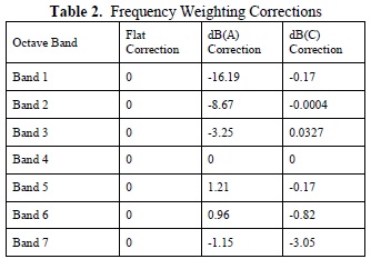
After performing all the calculations, the results are printed in the graphic user interface, with the option of three different frequency weightings (see Table 2) — flat, db(A), and db(C) — in order to correspond with the most used and required weightings in international acoustic standards.

4. Measurement procedure

The measurement procedure was carried out with an omnidirectional source which emits pink noise at a height of 1.5 meters above the floor. The input transducer was located at the same height at a distance of 1m from the acoustic center of the source and at a separation of 5cm from the capsule of the SLM's input transducer in order to attain the greatest recording correlation between the two systems.

Calibrations must be performed on both the capture system and the SLM to have the required values of pressure and RMS pressure as a reference. We then performed ten-second measurements with the source turned on and turned off and with the same capture signal time⁴.

Upon completing the measurements, we obtained results for the two and perfomed the necessary respective comparisons, as seen in the following section.

5. Results

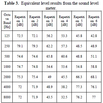
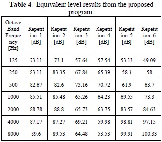
The results obtained under the aforementioned procedure are shown in the tables below. Table 3 shows the equivalent levels for each octave band determined by the SLM in a flat frequency weighting and a fast time weighting. Table 4 shows the results of equivalent levels from the proposed program for the determined octave bands. The tables show the data obtained under six repetitions using the same hardware for data acquisition.

6. Analysis of results

In light of Tables 3 and 4 of the previous section, one instantly sees that the equivalent SPLs per octave band from the SLM do not correspond to the equivalent SPLs from the proposed program. Thus, we took the decision of creating a table of the linear differences between the results (Table 5) to better observe the behavior of the systems.

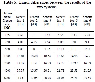
In Table 5, we can see in the differences between the results of both systems that the first four repetitions show a similar level of difference in almost every octave band. However, as the repetitions increase, the range of difference significantly increases as well.

In light of Table 5 and the above paragraph, we can consider the following possibilities for the cause of systematic error between the two results:

• The first and most important of the systematic errors in the project is the sound level meter, which has not been electronically calibrated in more than six years. This constitutes a rather large error in the calibration performed with the pistonphone (which, it should be clarified, has also not been electronically calibrated in the same period of time) and in the subsequent results of formal measurements of the signal of interest. This parameter constitutes an error of ±3 dB, which represents a 100% error in the limit values of the analysis (103 dB and 97 dB) of linear pressure in pascals. As a result, the main system error lies in the comparison of the results of the SLM which was used for the measurements.

• The calibration of the SLM (through the pistonphone) was performed only once, at the very beginning of setting up for project measurements. An error of 1.2 dB is evident in the calibration measurement, but this process was not repeated for the other measurement repetitions. It is possible that this error lightly influences the results, but given this possibility, it should be mentioned in order to mention all possible variables that can affect the final results.

• As the repetitions increase, one observes an increase in the differences of the results of the SLM versus the proposed program. The first three repetitions exhibit quite similar differences between them, but as the recordings increase, an increase in the differences between the results of the two systems is evident. This can be explained by the above error or by an error in signal flow in the external sound card, which undergoes temperature change during its use and can therefore affect the results displayed in the software (as in the aforementioned algorithms).⁵

• The large difference in the results obtained in the high frequency bands may implicate the error in numeral (i). Additionally, a "coloration" of the signal is evident, surfacing in the pre-amplification stage of the interface or the external card. Both phenomena must be considered, in addition to the uncertainty of the measuring device (the SLM), which shows errors of analysis when increasing the analyzed frequency.

6.1. Post-Processing Algorithm for the Proposed Signal

In light of Table 5 and the previously suggested errors, we propose a final correction for the equivalent level results of the proposed program. The objective of the proposal is to correlate the acquired data as much as possible between the SLM and the programmed system. It should be clarified that this post-processing of the results depends directly on the SLM with which one is comparing the data, and for this reason the suggested differences below will vary if a comparison is performed with a different SLM.

The proposed post-processing involves distinct, repeated measurements (5 or more if possible) by the SLM and the program in different arenas and acoustic environments. Next, one must examine the linear differences of the octave band equivalent levels for both systems, and calculate the average of correction of results for the proposed system. This guarantees the correlation of measured data from the SLM and results from the proposed program.

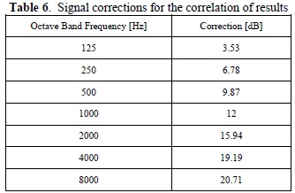
After applying these corrections to the results SLM (which is our reference quality system). These results can be seen in Table 7.

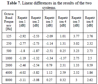
After applying the signal correction algorithm to increase the correlation of the results of the two systems, one sees in Table 5 that the maximum range of error was 4 dB and the minimum was 0.25 dB. With this, our system can produce values which correspond to the quality reference established by the SLM and which can be used to provide a solution for students and their need for a SLM during their learning process.

7. Conclusions

Our conclusions after completion of the project follow the above Results section and the Analysis of Results section.

Under the corrections established by the post-processing algorithm of the proposed signal in Section 6.1 and Tables 6 and 7, a considerably higher correlation between the results of the two systems (sound level meter and program) was achieved. We therefore conclude that by using as reference a SLM which has been electronically calibrated within the permissible period of time according to international standards and which is Type 1 or Type 2, a rather reliable system of capture can be attained with only the proposed algorithms and high-quality recording equipment.

Reflecting on the results of Table 7, we conclude that with the knowledge acquired at university (after around 2.5 years of study in the field of acoustics or sound engineering), one can program software for the acquisition and analysis of sound pressure level that is of the same quality as a commercial SLM, for use in academic testing and research projects.

Considering the method of software development proposed in this article, we conclude that the final result of the program and the concluding SPL results are directly linked to the reference SLM with which the measurements were performed.

It is critical, during the development of the software, to perform the proposed measurements again with a SLM which meets the criteria and quality requirements of international standards, in order to ensure the reliability of the results generated for the student by the proposed system.

The equipment used to perform the capture and recording of the signal to analyze must be specially constructed to perform field measurement work in order to avoid coloration and distortion of the natural acoustic signal recorded in the process, from signal flow all the way to entering the software analysis system.

The proposed system is only able determine equivalent sound pressure levels per octave band and an overall equivalent level of the recorded signal. Yet, with the knowledge acquired after two years of study in the field of acoustics, it is possible to develop analysis software replete with time weighting by frequency, with much narrower bandwidths, and which studies SPL decay in relation to the time, discretizing the behavior of the signal by relevant frequencies of analysis.

Acknowledgements

This study could not have been completed, nor could the analysis have been performed given the wide array of variables influencing the results, without the time and knowledge imparted by the physicist Alexander Ortega (ex-professor of Acoustics and Psychoacoustics at the University of San Buenaventura Bogotá campus), by Luis Fernando Hermida (MSc, current professor and director of the

Applied Acoustics research group at the same university), Shimmy García (Engineer and current professor of programming languages at the same university), Paula Tatiana Noreña (Engineering Physicist and current professor of Acoustic and Psychoacoustics at the same university), and everyone else who directly or indirectly influenced the production of this research project.

Notes

¹ See Fourier series and transforms
² Frequency used in the calibration.
³ See Table 1 for the lower and upper frequency limits of analysis by octave band octave band.
⁴ It must be noted that the measurement time is relatively the same, except for systematic errors derived from human reaction time (±35 milliseconds) and the reaction time of the computer used (no estimate). The performed measurements can be considered to have the same period for the two systems, since the systematic error is less than 1%.
⁵ This error should be considered reactive and thus does not constitute the same grade of error for low frequencies as for high frequencies.

References

[1] UNE- ISO International Organization for sandardization, «Ergonomics - Danger signals for public and work areas - Auditory danger signals (ISO 7731:2003),» ISO, 2003.         [ Links ]

[2] L. Beranek, Acústica, Madrid: Editorial Hispano Americana, 1969.         [ Links ]

[3] ISO- UNE ISO 1999:2008, International Organization for sandardization, «Determinación del nivel de la exposición al ruido en el trabajo y estimación de las pérdidas auditivas inducidas por el ruido(UNE 74-023-92).,» ISO, 2008.         [ Links ]

[4] D. Hattis, «Occupational Noise Sources and Exposures in Construction Industries,» Human and Ecological Risk Assessment: An International Journal, vol. 4, nº 6, pp. 1417-1441, 1998.         [ Links ]

[5] International Electrotechnical Commission IEC, «IEC 61672: Normativa para sonometros que consta de tres partes.,» IEC, 2002.         [ Links ]

[6] M. Nakatani, D. Suzuki, N. Sakata y S. Nishida, «A Study of Auditory Warning Signals for the Design Guidelines of Man-Machine Interfaces,» Human Interface and the Management of Information. Information and Interaction, 2009.         [ Links ]

[7] B. Pueo, Electroacústica: Altvoces y Micrófonos, Buenos Aires: Pearson Educación, 2003.         [ Links ]

[8] ISO- International Organization for standardization, «ISO 7731:2003 señales de peligro para lugares de trabajo. Señales acústica de peligro.,» ISO, 2006.         [ Links ]

[9] L. Bell y D. Bell, Industrial Noise Control: Fundamentals and applications, Second Edition, Lakewood: Hippo Books, 1193.         [ Links ]