


Serviços Personalizados
Journal
Artigo
 Inglês (pdf)
 Artigo em XML
 Referências do artigo
 Enviar este artigo por email
Indicadores
-
 Citado por SciELO
 -
 Acessos
Links relacionados
-
 Citado por Google
 -
 Similares em
SciELO
Similares em
SciELO -
 Similares em Google
Compartilhar

 Permalink
Tecciencia
versão impressa ISSN 1909-3667
Tecciencia vol.11 no.20 Bogotá jan./jun. 2016
https://doi.org/10.18180/tecciencia.2016.20.7
DOI: http://dx.doi.org/10.18180/tecciencia.2016.20.7
Comparative analysis between SOM Networks and Bayesian Networks applied to structural failure detection
Análisis comparativo entre redes SOM y redes Bayesianas aplicado a la detección de fallas en estructuras
Mauricio Pedroza Torres1*, Efraín Mariotte Parra1, Jabid Eduardo Quiroga1, Yecid Alfonso Muñoz2
1 Universidad Industrial de Santander, Colombia
2 Universidad Antonio Nariño, Colombia
* Corresponding Author. E-mail: ptorres.pro@gmail.com.
How to cite: Pedroza Torres, P. et al., Comparative analysis between SOM Networks and Bayesian Networks applied to structural failure detection, TECCIENCIA, Vol. 11 No. 20, 47-55, 2016, DOI: http://dx.doi.org/10.18180/tecciencia.2016.20.7
Received: 13 Oct 2015 Accepted: 18 Feb 2016 Available Online: 29 Feb 2016
Abstract
In this paper is carried out a comparative study between Self-Organizing Maps (SOM) and Bayesian Networks, to evaluate their performance in the field of structural health as damage detector of structural failures type III, which detects where the damaged area is and percentage of damage within this the area. The implemented classifiers are trained to detect structural failures in a simply supported beam and a truss of 13 elements, the detection is performed using modal information from different test scenarios, obtained by OpenSees® and MATLAB®. The simulations show a satisfactory performance of Bayesian networks to provide the range of stiffness variation in each element of the studied systems. Meanwhile, SOM networks are useful in predicting the decrease in elastic modulus, which is assumed as specific percentage of damage. Based on this results is proposed a hybrid methodology (BAYSOM) seeking to reduce computational cost and improve performance in diagnosis and detection of fault conditions in structures.
Keywords: (SOM) Self-Organizing Maps, Bayesian Networks, (SHM) Structural Health Monitoring, Damage Detection.
Resumen
En el presente artículo se realizó un estudio comparativo entre redes de mapas auto-organizados (Self-Organizing Map, SOM) y redes bayesianas, evaluando su desempeño en el campo de la salud estructural al determinar la ubicación y porcentaje de daño en fallas estructurales tipo III. Los clasificadores implementados se entrenan para monitorear una viga simplemente apoyada y una armadura de 13 elementos, esto gracias a la información modal de los distintos escenarios de prueba, obtenida mediante OpenSees® y MATLAB®. La simulación muestra un desempeño satisfactorio de las redes Bayesianas para suministrar el rango de variación en la rigidez de cada uno de los elementos bajo estudio. Por otra parte, las redes SOM se muestran útiles al estimar la reducción en el módulo de elasticidad de cada elemento, lo cual se interpreta como un porcentaje específico de daño. Con base en los resultados se propone una metodología hibrida (BAYSOM) buscando reducir el costo computacional y obtener un mejor desempeño en el diagnóstico y detección de condiciones de falla en estructuras.
Palabras clave: (SOM) Mapas auto-organizados, Redes Bayesianas, (SHM) Monitoreo de salud estructural, Detección de daño.
1. Introduction
Nowadays, it is not enough to determine the causes by which a structure may fail (fatigue, overloading, chemical degradation, etc.) it is just as important to implement an early detection of the fault conditions. Online fault detection systems must compensate the weaknesses of current methods in the detection of damage (X-ray, ultrasound, acoustic inspection, etc.) that require a priori knowledge of the possible fault location and a degree of accessibility to that location.
All approaches to Structural Health Monitoring (SHM), as well as all traditional nondestructive evaluation procedures can be cast in the context of a statistical pattern recognition problem [1]. In particular the vibration-based methods have received increasing attention in engineering structures.
Recently, ambient modal analysis techniques have focused on civil engineering structures since this technique is based on extracting the dynamics characteristics of a structure using ambient excitation (wind, traffic, loading, etc).
Assuming that modal parameters of a structure are available a fault detection system can be implemented tracking changes in local stiffness. In a deterministic SHM scheme, differences in the stiffness parameters estimated from different modal data sets would be used as indicators of damage [2]. Because of the complexity associated to regard all possible damage scenarios, probabilistic methods are required to consider uncertainties in the identified model by treating the problem within a framework of plausible inference in the presence of incomplete information [3].
Another approach available for SHM is SOM methodology, the architecture and the training of a neural network depends on which level of damage identification is required [4], but it appears that often simple unitary networks are not enough for complex pattern recognition tasks. In such cases networks can be combined, using different approaches [5].
Previously SOM and Bayesian networks have been implemented in the field of SHM [2, 5, 6, 7, 8, 9, 10, 11], but generally these techniques have been used as a complement of other methodologies. In [6] a SOM network is considered as an accurate classifier of different kind of fault, after a detection stage. Also, SOM networks are used to reduce the number of input signals without reducing the classification accuracy required [7].
Although, Bayesian Networks (BNs) are powerful tools for knowledge representation and inference under uncertainties in [8] is claimed that BNs present an acceptable performance as classifiers in SHM systems. In [9] BNs have been complemented with other concepts to structural damage localization by using of modal strain energy and frequency data, but the damage quantification continues to be a challenge. In order to reduce the high computational cost that a successful prediction entails, a simplified approach is required, seeking a successful methodology with a less computational cost.
In this paper, a comparison between SOM networks and Bayesian Networks is presented. Both approaches are used as fault predictors in two structures. Simulations show pros and cons of SOM networks and Bayesian networks as fault diagnosis systems. Finally, a novel approach BAYSOM is proposed to improve detection and quantification of structural damage.
2. Theoretical Framework
2.1. Dynamics of Structures
The structural dynamics theory states that an undamped structure with multiple degrees of freedom has a simple harmonic movement without changing the shape of deflection, this information consists of N natural frequencies, ωr, and N vibrational modes, Ψr ∈ RΝo, where Νo represents the number of degrees of freedom. These modal parameters can be analytically determined in the system in time domain, using (1):

Where ƒ,Χ ∈ RΝo and M, C,K ∈ RΝoΧΝo. The mass matrix is assumed known with sufficient accuracy from the definition of the structure, it is common to neglect the damping matrix in civil structures, and the stiffness matrix can be determined via the values of elastic modules in the structure.
2.2. Structural Health Monitoring
Structural Health Monitoring (SHM) is a technique to monitoring the condition of structural systems using the dynamic information of the excited system. Data are captured from a non-destructive sensor network to produce fault indicators to detect anomalies (damage or degradation) caused by deterioration, corrosion, fatigue, chemical reactions, moisture, changes in environmental variables and physical properties, stress, displacements, strains, vibrations, or dislocations in the structure.
Changes in the spatial model (defects) produce observable variations in the dynamic response of the system, the diagnosis algorithms are based on tracking those fluctuations along the structure. The fault condition in the system is obtained comparing the dynamic response of the healthy system with the damaged structure.
2.3. Bayesian Networks
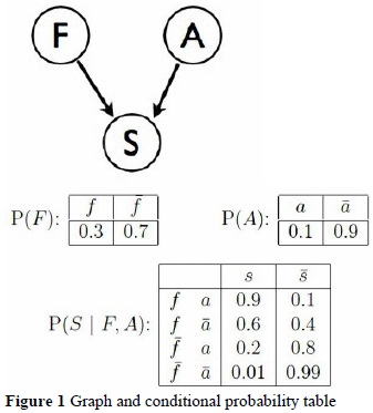
A Bayesian network is a directed acyclic graph where nodes correspond to random variables and arrows correspond to the direct influence of one variable on another. For discrete random variables, this conditional probability is often represented by a table, listing the local probability that a child node takes on each of the feasible values - for each combination of values of its parents. The joint distribution of a collection of variables can be determined uniquely by these local Conditional Probability Tables (CPTs).
BNs are both mathematically rigorous and intuitively understandable. They enable an effective representation and computation of the Joint Probability Distribution (JPD) over a set of random variables [12]. Although the arrows represent direct causal connection between the variables (Fig. 1), the reasoning process can operate on BNs by propagating information in any direction.
A Bayesian network represents a Joint Probability Distribution ( JPD) between its variables X1, …, Xn by means of the chain rule for BNs (2):
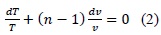
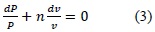
Bayesian Networks provide a compact method to specify the joint distribution of a cluster of variables. The probabilistic terms used inBNs approach are:
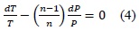
"A priori" probability: It is the absence of evidence. Knowing "a priori" probability of x and the conditional probability P (y1&luml; x) is possible to calculate the probability of y1 by the total probability theorem, as shown in (3):
"A posteriori" probability of X when available evidence " e" is calculated as (4):
Given the evidence e= {yi}

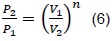
We can see it in standard form in (6):
Where: λy(x) = αP(elx)= P(ylx) and α = [P(e)]−
As some variable values are known, it is possible to update the value of the rest of the variables. The inference is the process to introduce new observations to calculate the new probabilities for the rest of the variables. Therefore, the inference process corresponds to a posteriori probability P(Xly)= Xi of a set of variables X for a set of observations Y =yj where "Y" is the list of observed variables and "yj" corresponds to the observed values:
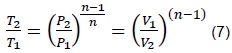
The probabilistic networks operate using the Bayes’ theorem expressed in (7) as:
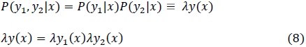
According to Bayes’ theorem given e= {y1, y2} applying conditional independence in (8):
Bayesian Networks provide two types of inference support: predictive support for node Xi, based on evidence nodes connected to Xi through its parent nodes (also called top-down reasoning), and diagnostic support for node Xi, based on evidence nodes connected to Xi through its children nodes (also called bottom-up reasoning) [13].
The BN learning problem, which can be stated as follows: Given training data and prior information (e.g., expert knowledge, casual relationships), estimate the graph topology (network structure) and the parameters of the JPD in the BN. The learning is performed assigning a prior probability density function to each parameter vector and use the training data to compute the posterior parameter distribution and the Bayesian estimates.
2.4. Self-Organizing Maps (SOM)
A self-organizing map (SOM) is a type of neural network trained using unsupervised learning to produce a n-dimensional, discretized representation of the input space of the training samples, called a map. The map can be described as an array of elementary processors (i,j) arranged in two dimensions, which store a synaptic weight vector Wij (t), where {Wij(t); Wij ∈Rm 1≤i ≤ nx, 1 ≤j≤ ny}.
SOM operate in two modes: training and mapping. Training builds the map using input examples; it is a competitive process, also called vector quantization, whilst mapping automatically classifies a new input vector according to that map. A self-organizing map consists of components called nodes or neurons, in which each node is a weight vector of the same dimension as the input data vectors and a position in the map space. The first step in the procedure for locating a vector from data space onto the map, it’s to obtain the node with the closest weight vector to the data space vector. Once the closest node is located it’s assigned the values from the data space vector.
The objective of training in the SOM is to produce different elements of the network which respond similarly to certain input patterns. The weights of the neurons are initialized to small random values. The training uses competitive learning, when a training example, input vector x, {xk ∥ 1≤ K ≤ m} and its own synaptic weight vector Wij is fed to the network, its Euclidean distance or another criterion of similarity to all weight vectors is computed, as shown in (9):

The neuron with weight vector most similar to the input vector is called the Best Matching Unit (BMU). The weights of the BMU Wg and neurons close to it in the SOM lattice are adjusted towards the input vector. In this manner, each neuron acts as a detector of specific behavior, and the winning neuron indicates the kind of features or pattern detected in the input vector. During training the SOM network is a static network that tends to take the shape of the cloud of data (training set).
In the learning phase each neuron of the map tuned to different ranges of the input space. The SOM network usually consists of a two-dimensional grid of map units, each map unit i is represented by a prototype vector mi = [Mi1, ....,Mid] where d is the size of input vector, each unit is linked to the adjacent through neighborly relations. The process is as follows: SOM network are trained iteratively, in each training step the distance between a sample vector x of the training set and the vectors of grid of map units are calculated and also the Best Match Unit (BMU), which is denoted by b is mapped unit closest to the prototype vector x:

Prototype vector is updated, the BMU and its topological neighbors are moved closer to the input vector in input space, the update rule for vectors is:

Where t is the time, Α(t) is the adjustment coefficient, hbi (t) is the centering function of the winning unit:
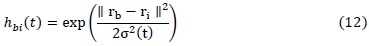
Where rb and ri are the position of b and i neurons in the SOM network. Both functions α(t) and (t) σ(t) decrease in time.
The error can be observed from the following expression:
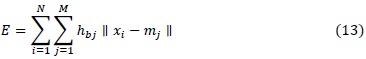
Where N is the number of training iterations and M is the number of map units.
The neighborhood function hbi is centered in the unit b, which is the BMU of the input vector xi, and is assessed on each unit j.
3. Analyzed Structures
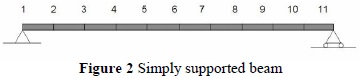
In this paper, a simply supported beam and a truss are used to evaluate the performance of the SOM and BNs in fault detection and diagnosis. The parameters of the beam, shown in Fig. 2, are: length L=6 m, equally discretized in 10 elements, as shown in Figure 2, A= 0.12 m2, Iz=1.6x10⁻³ m4, built in concrete of 3000 Psi, E= 2.153x10¹⁰ Pa, and mass per unit volume = 2402.769 kg/m3.
In Figure 3 is shown the truss used in this study. The parameters of the truss are: 13 elements, with a height of 2.4 m and a total length of the base of 7.28 m, horizontal elements of 1.82 m of length are evenly spaced, as shown in Figure 3, A= 4x10⁻⁴ m2 and steel material A-36 with E=2.0x10¹¹ Pa.
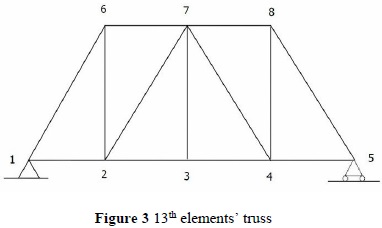
The beam and the truss were discretized as shown in Figures (2-3). OpenSees® software is used to analyze and describe the dynamic behavior, which is condensed in a vector αi . The vector contains the first four αi natural frequencies and the vibrational modes of the analyzed structures represented as the position in the vertical axes of each node in the 2-d graph shape of each mode.
4. Implementation and Experimentation
The dynamic responses of the structures, frequencies and modal information, are determined using the free software OpenSees®. Using the follows information:
- Reductions of E (Elastic modulus) between 0- 30%.
- Linear response of the structure.
- No damping is considered.
For the study of the fault conditions, the damage is emulated in MATLAB® decreasing the value of E in one or multiple elements of the structure. This new version of the structure is introduced in OpenSees®, for determining the dynamic response. This information is used for training propose and validation using the SOM and BN approaches. In the case of the beam and the truss, the input vector includes modal information of the first four vibrational modes of the structure, as it was described in [14].
Since, SOM networks provide the probable E values for each element of the structure and BNs determinate the most probable damage category of this element; different indicators are used for performance evaluation of SOM and Bayesian networks.
4.1. Bayesian Methodology
A new approach is proposed using BNs for monitoring the structure. The predictive procedure is implemented in MATLAB® environment.
The Bayesian network is trained to obtain the parameters such as: nodes, connections and probabilistic parameters. The Bayesian inference algorithm provides the probability values of damage occurrence on each element of the structure for each test scenario.
Parametric Training
- The entry vector αi is organized as follows in (14):
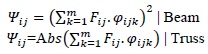
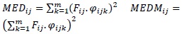
- A parameter Ψij based on the modal information is determined to label each damage scenario:
- The vectors Vij are arranged in a matrix Mj organized according to Ψij, where vectors Vij with higher numerical values of Ψij are translated to the top of the evidence matrix Mj, for instance:
- Conditional Probability Table (CPT).
- The Bayesian network structure is determined with the definition of structural elements as parents and ranges of probabilities values as children. The training corresponds to the information contained in the CPT’s, which provides the probability values to its related evidence node (probabilistic parameters).
- The classification process of a new input vector in the most probable CPTs is performed by the value of Ψij, the classification actives the evidence node related with each CPTs where the new input vector is stored, which allows to obtain probabilities about presence of damage in each analyzed element using Bayesian inference.

Where i is the damage scenario, n represents the number of analyzed scenarios, Fij is the natural frequencies of each damage scenario i in each vibrational modes j and Φij is a vectors for each vibrational mode containing the displacements φijk of the nodes, where k varies from 1 to the total number of nodes m. The vector αi is linked with the damage distribution βi (15).

and E in normal conditions, where h varies from 1 to the number of elements of the structure (e). Additionally, vector βi is simplified to a binary form (£i), where Xih is changed by Sih where:
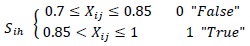
Where "false" denotes damage
The simplified vector £i is shown as follows in (16):

Then a new vector for each mode of vibration is created as follows in (17):

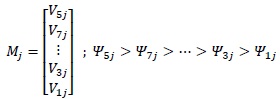
This matrix Mj is divided in a z number of evidence submatricesNjz according to numerical proximity between Ψij values:
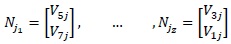
The z value depends of the number of evidence nodes that will be used in the Bayesian network, because each evidence sub-matrix originates one conditional probability table, which is related with one evidence node.
The CPT matches the damage probability of the element to its neighborhood elements trying to recreate a real situation of dynamic response variations around the location of the fault. This organization creates 3 graphs to reduce the complexity of the calculation of a posteriori probability
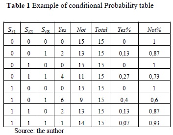
Each table contains information of its corresponding submatrix Njz. The table is organized according to the different combinations of damage based on the Sie values, so each combination of damage has associated a number of ξi vectors. Then, it is possible to correlate the fault condition with the Ψij values, used as reference in the construction of the CPT.
4.2. SOM Methodology
In this research the U matrix is used to evaluate the SOM training. The U matrix indicates the synaptic weights of the neural network as a distance from one neuron respect to another, showing the training quality of the network, the error rate of proximity and finally, the position of the winning neuron. SOM approach is implemented as follows:
- Generation of the training set, with random damage scenarios in the complete structure (total uncertainty).
- Setting the feature vector using modal information for each fault scenario, including the Minimum Euclidean Distance (MED) and a second criterion as follows::
- Reorganization and normalization of eigenvectors and eigenvalues as the training set.
- Labeling the vectors of each scenario with the corresponding damage scenario for each element (percentage of damage assigned to each element).
- SOM training using U matrix, the quantization error and topological error as a performance criterion.
- Validation.
- If the response of the trained SOM to the validation set is not acceptable a new training is performed varying training parameters such as: time in ages, topology, size, unit radio.
A set of 1000 cases of study are used for training process. Each case of training corresponds to a faulty condition. Fault conditions in the structure are emulated varying the number of damaged element and the level of severity.
In order to assess prediction capabilities a set of validation is used. Each faulty scenario is tested 6 times to verify the repeatability of the proposed SOM network after the training stage.
5. Simulations and Results
5.1. Bayesian Results
The performance of the proposed Bayesian network is evaluated using the following criteria:
- Significant damage [0.7 E-0.85E].
- Tolerance range [0.83 E - 0.88E].
The experimental results are shown in Figures 4, where significant error is when the fault condition is identified but the damage value is out of the tolerance range, negative false, if the element is assumed without damage when the fault condition is presented, and serious errors, when the negative false prediction exhibits high damage values.
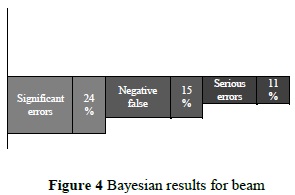
A training set of 1000 damage scenarios is used in the training stage. In Figure 4 is shown the statistical behavior of the Bayesian prediction using the cross-validation set composed by 50 different structures under diverse damage conditions
5.2 SOM Results
In this study x denotes the relation between the simulated E and E in normal conditions. Additionally a faulty condition is considered if 0.7 ≤ x≤ 0.85, and an undamaged element if 0.85 < x ≤ 1.
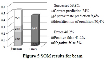
A correct prediction is assumed when x calculated is around of + 0.03 from real value of x, and an approximate prediction if it ranges + 0.05, identification of condition (only fault condition is identified), positive false (prediction of damage in an undamaged element), negative false (prediction of healthy condition in a damaged element).
The SOM methodology is susceptible to be affected by duplicity in the dynamic response, i.e. the same dynamic response for a different fault scenario. Therefore, SOM performance depends on the ability to limit the range of values where network can be trained.
Figure 5 shows the low performance of the SOM network evaluating the condition of different scenarios in this case is shown the statistical behavior in the diagnosis of 50 different damage scenarios.
As described above SOM and Bayesian networks present a relatively acceptable performance in fault detection and diagnosis in structures using the dynamics characteristic as a fault indicator. A novel approach BAYSOM is proposed to enhance the fault detection and diagnosis performance based on the advantages associated to SOM and Bayesian networks.
6. Baysom a new Approach
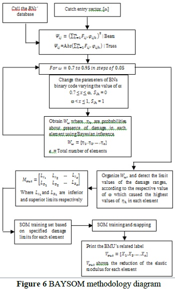
In this novel approach the fault detection system is divided in two stages. In the first stage, the BNs is used to predict the element under fault condition and estimates the range of variation of the elastic modulus E, this process is conducted as it was specified in BNs’ Training, but probabilities about the presence of damage in each element are modified to the most probable range of E variations (where that element is located). The first stage is achieved because the criterion used for simplification from vector βi to vector ξi can be manipulated, for instance: if 0.7 ≤ x <0.75, then Sih = 0, and if 0.75 < x ≤ 1, then Sih = 1. The process of variation in the simplification criterion provides the range of E variations with the highest probability values for the analyzed element. In the second stage, the SOM network is fed with the intervals obtained in the first stage to predict the change of E.
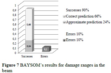
BAYSOM network is evaluated following the next criteria:
- Correct prediction (real damage value, located into the range).
- Approximate prediction (real damage value, located to ± 0.03 to range limit).
- Error (real damage value, out of range).
In Figure 7 can be observed the results obtained using the first stage of the BAYSOM approach. In this Figure is noted the performance of the proposed methodology in determining the faulty element and the variation range E.
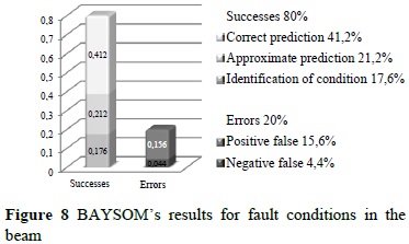
As shown in Figure 8 the correct prediction of BAYSOM methodology is promising compared with SOM and Bayesian networks dealing individually, achieving an 80% of success in the detection of the fault conditions. Although the percentage of errors is around 20% only less than 5% correspond to negative false.
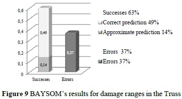
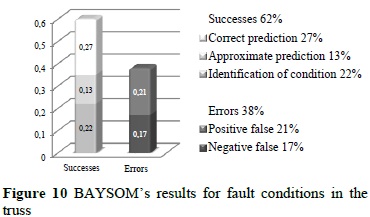
In Figure 9 can be observed the prediction of the implemented approach used in the truss. Simulation results in Fig. 10 shows a reduction in performance of the BAYSOM fault detection system, this phenomenon can be attributed to a limited number of training cases available for describing the complete dynamic response (greater amount of damage scenarios) due to the high dynamic complexity of the truss.
7. Conclusions
In this paper, a fault detection system for a truss and a beam is studied. A Bayesian network and a SOM network are used for fault location and fault severity estimator. Simulations show a computational time ratio of around 2:1 between Bayesian network and SOM trainings. The experimental results for the beam show success rate of 53.8% for SOM network and 66% for Bayesian network respectively. The results obtained for the truss were not considered because the poor performance of both approaches. So, as a conclusion, the use of a simple approach i.e. SOM or Bayesian networks presents an inadequate performance as predictors of the actual condition of the studied structures.
Based on the mentioned above, a novel approach is proposed, the BAYSOM methodology, which combines the ability of Bayesian inference to obtain the most probable ranges of damage value with the SOM network’s ability to find the closest value of E variations using a trained database.
In the case of the beam, the success rate obtained by implementing the BAYSOM methodology is 90% for range identification and 80% for damage value estimation. For the truss the success rate is 63% for range identification and 62% for damage estimation. Therefore, a reduction of performance is presented as complexity of the structure increases. In order to improve the operation a more extended database is needed.
Based on simulation results, high hits percentage, and its low computational cost BAYSOM can be considered as an efficient theoretical approach in the field of simulation and detection of structural faults.
References
[1] Farrar CR, Doebling SW, Nix DA, Vibration-Based Structural Damage Identification. Philosophical Transactions of the Royal Society: Mathematical, Physical & Engineering Sciences, 2001; 131-149. [ Links ]
[2] Vanik MW, Beck JL, Au SK, Bayesian probabilistic approach to structural health monitoring. Journal of Engineering Mechanics; 126 (7): 738-745. [ Links ]
[3] Cox RT. The algebra of probable inference, Baltimore: Johns Hopkins University, 1961. [ Links ]
[4] Rhim J, Lee SW. A neural network approach for damage detection and identification of structures. Computational Mechanics; 16: 437-443. [ Links ]
[5] Marwalla T. Probabilistic fault identification using a committee of neural networks and vibrational data. America Institute of Aeronautics and Astronautics, Journal of Aircraft; 38 (1): 138-146. [ Links ]
[6] Yuan S, Wang L, Peng G. Neural Network Method Based on a New Damage Signature for On-Line Structural Health Monitoring. Nanjing: Nanjing University of Aeronautics and Astronautics, 2003. [ Links ]
[7] Kolakowski P, Mujica L, Vehi J. Two Approaches to Structural Damage Identification: Model Updating versus Soft Computing. Journal of Intelligent Material Systems and Structures; 17 (1): 63-79. DOI: 10.1177/1045389X06056073. [ Links ]
[8] Addin A, Sapuan S, Mahdi E, Osman M, Ismail N. Bayesian network approach to classify damages and f-folds feature subset selection method in laminated composite materials. Serdang: Universiti Putra Malaysia; 3-6. [ Links ]
[9] Huiyong G, Zhengliang L. Bayesian Fusion Theory and its Application to the Identification of Structural Damages. Fourth International Conference on Natural Computation; 4: 110-114. [ Links ]
[10] Sofge DA. Structural health monitoring using neural network based vibrational system identification. Cambridge: NeuroDyne Inc, 1994; 91-94. [ Links ]
[11] Tamminen S, Pirttikangas S, Röning J. Self organizing maps in adaptative health monitoring. Oulu: University of Oulu. Machine Vision and Media Processing Group, 1999; 1-6. [ Links ]
[12] Pearl J. Probabilistic Reasoning in Intelligent Systems. San Francisco: Morgan Kaufmann. 2ed, 1988. [ Links ]
[13] Ben-Gal I. Bayesian Networks. Encyclopedia of Statistics in Quality and Reliability, John Wiley & Sons. Ruggeri F., Faltin F. & Kenett R. (Eds.), 2007. [ Links ]
[14] Ramirez D, Gómez I, Quiroga J. Structural damage detection using PSO optimization technique. Ingeniería y Desarrollo; 28: 89-101. [ Links ]
[15] Andrew Ng. CS229 Machine learning: Lecture notes unsupervised learning [online]. 2010. Disponible en internet: http://www.stanford.edu/class/cs229/notes/cs229-notes7a.pdf. [ Links ]
[16] FullBNT-1.0.4 develop by Kervin Murphy at the California University, Berkeley. [ Links ]
[17] SOM Toolbox Version 2.0 beta, programed on MATLAB® and developed by por Esa Alhoniemi, Johan Himberg, Juha Parhankangas y Juha Vesanto. [ Links ]
[18] M. Pedroza, E. Mariotte. "ANALISIS COMPARATIVO ENTRE REDES SOM Y REDES BAYESIANAS APLICADO A LA DETECCION DE FALLAS EN ESTRUCTURAS". B.S. thesis. Dept. Mech. Eng., UIS. Bucaramanga, STD, 2011. [online] avaible: http://tangara.uis.edu.co/biblioweb/. [ Links ]

