DOI: http://dx.doi.org/10.18180/tecciencia.2016.20.10.

Non-Traditional Flow Shop Scheduling Using CSP

Scheduling Flow Shop No Tradicional Empleando CSP

Juan Pablo Orejuela¹, Andrés Felipe León Díaz^1*, Alexander Suarez Riascos¹

¹ Universidad del Valle, Cali, Colombia

^* Corresponding Author. E-mail: anfeledi@hotmail.com.

How to cite: Orejuela, J.; León, A.; Suarez A., Non-traditional flow shop scheduling using CPS, TECCIENCIA, Vol. 11 No. 20, 71-79, 2016, DOI: http://dx.doi.org/10.18180/tecciencia.2016.20.10.

Received: 09 Sep 2015 Accepted: 05 Feb 2016 Available Online: 29 Feb 2016

Abstract

This paper addresses the problem of scheduling in a flow shop manufacturing environment with non-traditional requirements, where some jobs must be scheduled earlier and others later depending on the priority established by the demand characteristics supplied. The problem is formulated mathematically, and given its nonlinearity, we propose a CSP (Constraint Satisfaction Problem) model, which is formulated using constraint programming with the software OPL Studio®. A set of experiments was performed by varying the weighting of jobs. We also varied the deadlines and waiting times among the machines. Finally, different production schedules were attained according to the type of experiment, thus solving the problem of non-traditional scheduling.

Keywords: Scheduling, Operations Programming, Flow-shop Manufacturing Environment, Constraint Programming.

Resumen

En este documento se aborda el problema de Scheduling en un ambiente de fabricación Flow-Shop con requerimientos no tradicionales, en el cual algunos trabajos deben ser programados en su momento más temprano y otros en su momento más tardío dependiendo de la prioridad establecida por las características de la demanda a suplir. El problema es formulado matemáticamente y dada su no linealidad se propone un modelo CSP (Constraint Satisfaction Problem) para su solución, el cual se formula mediante programación por restricciones utilizando el software OPL studio®. Se realizaron un conjunto de experimentos, variando la ponderación de los trabajos, así mismo se variaron la fecha de terminación y los tiempos de espera entre máquinas. Finalmente, se obtuvieron diferentes programas de producción acorde al tipo de experimento dando una solución al problema del Scheduling no tradicional.

Palabras clave: Programación De Operaciones, Scheduling, Ambiente De Fabricación Flowshop, Programación Por Restricciones.

1. Introduction

Scheduling seeks to assign sequence and schedule production orders. This problem is combinatorial, and its domain grows exponentially as a function of the variables, which makes the problem highly complex (NP-Hard). According to [1] there are two types of techniques to scheduling: approximation methods and optimization methods.

Approximation methods: These are divided into four categories a) priority dispatch rules, b) bottleneck-based heuristics, c) local search methods, and d) artificial intelligence [1]. Among the latter we find constraint programming, which can also be divided into two branches: constraint satisfaction and constraint solving. Constraint satisfaction deals with finite domains, while constraint solving is focused on infinite domain or more complex domain problems [2].

Optimization techniques: An optimal solution is built from the problem data by following a set of rules that precisely determine the processing order [3]. Some scheduling problems are solved effectively by these techniques. However, its algorithms can become computationally too complex, which makes approximation techniques an interesting strategy.

One of the most useful approximation techniques currently used to solve scheduling problems is Constraint Programming (CP), which uses constraint satisfaction to explore the search space and to obtain a solution, eliminating from the sets of variables all those values that cannot be part of a solution to the problem. Following we present some research regarding the use of this technique in the scheduling problem and other similar problems.

In [4], a combination of three models of mixed integer programming is compared to the CP model in order to solve a real assembly scheduling problem with constraints on inventory and a set of machines. Here, the objective is to minimize the weighted delay of all orders. Constraints guarantee the release and completion dates of the activities and the delay of each order, as well as machine capacity, which can only process a single unit in a certain time. Moreover, [5] deals with the Quay Crane Scheduling Problem (QCSP), which consists of programming quay cranes for unloading tasks on a ship. A CP model is proposed, with constraints on time, space and the use of cranes. The objective function seeks to minimize the makespan.

Furthermore, [6] presents a solution to a problem of production and distribution of newspapers. The authors propose a CP model for a routing problem with time windows and zoning constraints. It has a sequence in production and a sequence in distribution, where the latter depends on the first. They are subjected to capacity and availability constraints on cargo trucks, limitations on coverage distance for the trucks, and time windows for deliveries. The aim is to minimize the distance covered by the trucks, solving the constraints of the problem.

In [7] we find a model to solve a scheduling problem with a determined number of jobs to be processed on a machine, subject to the deterministic availability of the machine. All jobs must be processed on a single machine and the goal is to minimize the flow time of all jobs, according to the availability constraints of the machine. We find more research on CP models, with scheduling solutions to problems in different environments [8] [9] [10] [11] [12] [13] [14] [15] [16] [17] [18].

The proposal presented in this paper seeks to address a Non-Traditional Scheduling problem using the paradigm of Constraint Programming (CP). The problem is thus presented in Section 2. In Section 3, a mathematical modeling strategy is presented, which shows the complexity and nonlinearity of the problem. In Sections 4 and 5 solution methodology is presented, and in Sections 6 and 7 we present the case study, the results, and finally, in Section 8, our conclusions.

2. Materials and Methods

2.1. The Problem: Scheduling with non-traditional requirements.

The scheduling problem is defined as the allocation and sequencing of a set of jobs J, in a resource set M, where each job comprises a series of operations O which use the resource set M. There is also a set of constraints R, which are associated with the resources and activities. When scheduling is performed, the product obtained is the dates when each of the operations of the job will be performed, also known as a schedule. In Flow Shop Scheduling the goal is to obtain a job sequence by optimizing a defined criterion (usually the makespan) in a fixed order through the machines.

The scheduling problem has been extensively studied in the literature, since it is complex and it is common in multiple industries and environments. Various researchers have addressed the issue from different perspectives and in different environments, where every feature of the environment creates new requirements and challenges [4], [19] [20] [21] [22].

2.1.1 Non-Traditional Scheduling

This paper presents a problem involving scheduling the manufacturing of a set of jobs over a time period i, to meet the demand for a time period j. The priority in the manufacturing sequence depends on the period in which the order is used to meet the demand. Production orders made to meet the demand from an earlier and/or current period are always programmed as early as possible. Moreover, production orders made to meet the demands of a future period should be scheduled as late as possible. Hence, what makes this a Non-Traditional Scheduling problem is the need to schedule some work or production orders as early as possible and others as late as possible. For this specific problem, the following variables are assumed to be known: some production orders of work k, to be manufactured in I, to meet the demand in j; OP_Kij.

The goal is for the jobs for immediate consumption (II) and pending jobs (I) to be manufactured as early as possible, since they must be delivered as soon as they are finished. This suggests that the role is to minimize the inventory of the product in process, which is equivalent to reducing the time of total flow. For priority jobs (III), the goal is to process them as late as possible so they do not remain long as a finished product. This is equivalent to minimizing the inventory of finished goods at the end of the line.

This situation is problematic because in failing to consider non-traditional requirements, orders meeting future demand would be manufactured too early, thus generating a cost for maintaining inventory, and, as a worst case scenario, it would cause a blockage on production due to a lack of storage space for finished products. Indeed, in [21] we find that the author presents a two-phase scheduling model. The first phase is for priority jobs I and II, where the goal is to process them as soon as possible, and the other is for priority jobs III, were the goal is to process them as late as possible. The author then attempts to solve this problem in one step, applying a single scheduling which has no traditional requirements, using CSP.

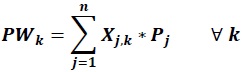
2.2 Initial Proposal: Linear-Programming Model

This paper uses the proposal in [23] as a starting point. For the case presented here, a variant was included which consisted in calculating the Total Flow Time (TFT) in terms of position k of the sequence s and multiply it by a PW_k variable, which corresponds to the weight of a job in terms of its position k and sequence s.

2.2.1 Linear programming Model

Parameters
Jobs (j): operations to be performed on machines.
Machines (q): resources for processing jobs. You can only process one job at a time.

Variables
X_j,k: Binary variable that takes the value "1" when the job j is assigned to a position k of a sequence
iiK_i,k: time the machine i remains idle, which occurs from after finishing job processing at position k until starting to process the job in position k + 1.
W_i,k: time waiting for a job at position k, which occurs from the moment it stops being processed on machine i, until it begins to be processed on machine i + 1.
C_k: completion of the last operation of job k.

2.2.2 Constraints

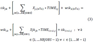
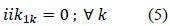
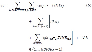
Where (1) and (2) ensure a single job per sequence and vice versa. Equation (3) ensures the functionality of the sequences, while (4) and (5) ensure that the first job on a machine does not wait and that the first machine does not wait. Equation (6) shows the date of completion of each job.

Since this problem requires managing the jobs by priority according to the features explained in the definition of the scheduling problem, Priority I and II jobs need to be scheduled as early as possible, and Priority III jobs as late as possible. For this purpose, the PW_k variable was included in the objective function to represent the importance of jobs in position k of the sequence.

2.2.3 Objective Function: Total Weighted Flow Time

In the objective function we observe its non-linearity, which renders difficult the use of integer linear programming techniques. Thus, to solve the problem, we have chosen the methodology CP, which uses elements of constraint satisfaction such as closure and constraint propagation to reach a solution.

2.3 Constraint Programming (CP)

The main idea of CP (Constraint Programming) is to use the knowledge of constraints to remove from the domain of variables the values that cannot be part of a solution. In this way, it is possible to solve a problem by reducing the domains of its variables until achieving very close approximations to the solution value [4]. A CSP (Constraint Satisfaction Problem) is a finite set of variables, each of which has a value domain, and there is a set of constraints that limit the combination of values that the variables can take [24].

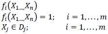
A CSP can be represented as a triplet (X, D, C), where:
X = { X₁, X₂, X ₃,…X_n }: a set of n variables.
D = { D₁, D₂,….D_n }: set of finite domains, where D i is the domain of X_i .
C = { C₁, C₂,….C_n }: finite set of constraints, where each constraint k-aria C_i constrains the values that the k-variable can take simultaneously. One particular case is the binary restriction, which relates only 2 variables, X_i and X_j and is known as C_ij.

For the scheduling problem, instantiation is identified. This means the variable-value relationship that represents the assignment of value a to the variable X (X = a). So the instantiation of a set of variables is a tuple of ordered pairs, where each pair (X_i, a_i) assigns a value {a_i∈ D_i } to the variable X_i. A tuple (( X₁, a₁ ), ( X₂, a₂ ),.....,(X_i, a_i ) is locally consistent if it satisfies the constraints formed by the variables {X₁, X₂,..., X_i } of the tuple; to simplify the notation of the instantiation of a set of variables, the tuple (( X₁, a₁ ),….,( X_i, a_i )) is replaced by (a ₁,…, a_i ).

A solution of a CSP is an assignment ( a₁, a₂,...a_n ) of values to variables, so that the constraints are satisfied. In other words, a solution is a consistent tuple containing all the variables of the problem, and a partial solution is a consistent tuple containing some of the variables of the problem. It is said that a CSP is consistent if it has at least one solution, meaning that it at least has a consistent tuple. Originally constraint satisfaction was applied only to find workable solutions. However, when constraint satisfaction is included in a more elaborate structure, it can also be applied to optimization problems, as shown: [25]

Minimize X_i (X₁…,X_n); Subject to:

Some of the applications where CSP is used to solve scheduling problems [26] [27] [28] [29] [30].

2.4 Model: Solution proposal

2.4.1 Sets
Jobs [j]: operations to be performed on each machine.
Machines [q]: resources for processing jobs (one job at a time).

2.4.2 Parameters:
Duration[j,o]: time that a resource takes to process an activity.
Operations[j,o]: set of activities that make up a job.
Weight[w_j]: value assigned to jobs in function of the degree of importance among them.
Ready time[r_j]: release date of job j.
Deadline[d_j]: time in which the job j must be completed.
tmp: maximum time that a mixture can be in process.

2.4.3 Variables:
Start (s_j, o): date on which the job j or operation starts.
End (e_j, o): date on which the job j or operation ends
Total weighted flow time (TWFT): the summation of the subtraction of the termination date, minus the ready time of each job multiplied by their respective weight.

2.4.4 Objective Function

Minimize:

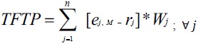
Where M is the machine where the last operation of all jobs is run.

2.4.5 Constraints
Precedence Constraint:
e_j,o ≤ S_j,o+1; ∀_j
Job release constraint
S _j,1 ≥ r_j; ∀_j
Delivery of jobs constraint:
e_j,o ≤ d_j; ∀_j
Machine capacity constraints: Max (e_j,i) ≤ cap_i; ∀_j
Maximum time of product in process constraint:
( e_j,3 - = S _j,1) ≤ tmp_j; ∀_j

2.5 Case Study - Animal Feed Industry

Our research focused on the scheduling phase, developed at the lower level of the hierarchy proposed in [21]. There are 3 machines operating 8 hours a day, 6 days a week and the manufacturing environment is a flowshop without storage between machines. Five weeks were scheduled (240 hours to schedule jobs).

2.5.1 Nature of the Products
The product was feed concentrate for chickens, laying hens and pigs. They are classified into two categories: Priority I and II (products manufactured to meet demands of past and current periods), and Priority III, which are products manufactured to be delivered at a later period. Every operation of every job is performed on a single machine and has a known duration. The parameter "weighting" was created, representing the priority of a job in terms of the period of its demand.

The weighting of a job is multiplied in the objective function by the time flow. Because the objective function is minimization, the model tends to always schedule the processing of jobs with higher positive weights (Priority I and II jobs) at earlier dates and the processing of jobs with negative weights (priority II jobs) at later dates.

2.5.2 Company’s scheduling problem
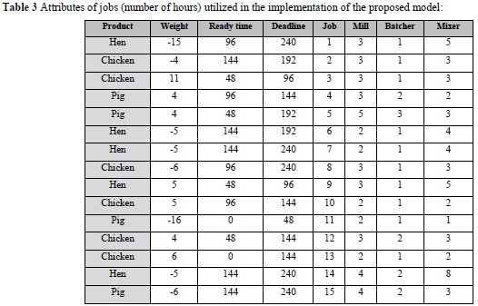
Table 1 shows product quantities for the periods of demand jand production periods i, which determines the deadline and ready time of the jobs.

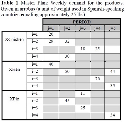
A job with a ready time of 0 is not always priority I. It is possible that a job is released on the zero date to supply a future demand and that it has a negative weight. Jobs with a ready time different than zero also may not be classified immediately as priority II, because it is possible for a job to be released on a date greater than zero and to be priority I; in other words, to have a high weighting and be processed at early dates.

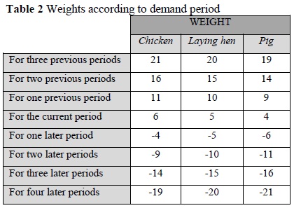
For jobs with demand in the same period we establish a priority according to the importance of the product. For example, in Table 2, for the case of three previous periods the weighting for Hen is 20. Since Chicken is more important, its weight is 1 value higher to denote such importance. Pig is less important, and thus is set as 1 value lower.

3. Results

Five experiments were performed. In the first, all jobs had positive weights. In the second, all jobs had negative weights. In the third, there were 8 jobs with positive weighting, and gradually the number of jobs with negative priority increased. In the fourth, the parameter tmp was not used; this means that once jobs began, the process could finish at any point. The fifth was called "no wait", because once it starts processing, the job could not wait to be processed in a machine.

3.1 Case 1

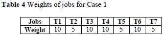
The model was run for one week (48 hours) with 8 jobs of positive weight (see Table 4), meaning that only demand from past periods (missing) and the current period are met. This case represents traditional scheduling.

Operations were processed as soon as possible. The time flow of the job and the inventory of the product in process were minimized (see Figure 1).

FIGURE 1

The last operation ends at u = 41 and not at the capacity limit u = 48. Machine 1 did not show idle time, while the other 2 machines did, because they had to wait for the operation that preceded them. Jobs did not have wait times on any of the 3 machines. To minimize the TWFT, the model tried to make the C_j as small as possible, so that jobs are processed as soon as possible.

3.2 Case 2

The model was run for a week (48 hours), with 8 jobs of negative weight (see Table 5), meaning that only future periods are demands met. All jobs are intended to be processed at the latest possible date.

The operations are processed as late as possible, with no operation scheduled at time zero. The goal is to minimize the inventory of finished products in the line. Jobs with higher weight - among the negative weights—were scheduled first. Machine 3 had no idle time and it was busy until the workshop closed.

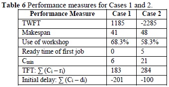
To minimize this indicator, the model makes Cj as large as possible, so that when multiplied by the negative weights, the product gets smaller and smaller. This explains why Priority II jobs are scheduled to be finished as late as possible. Table 6 shows performance measures for Cases 1 and 2.

The model was run 9 times, for 8 jobs. In the first run they all started with positive weighting and a ready time of zero. For each run jobs with negative weight were increased by 1. All jobs are of equal duration, so that it makes no difference which job is assigned the negative weighting. Table 7 shows the performance measures for the new runs.

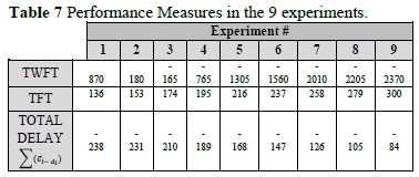
In the first run (#1) we find a traditional scheduling (there are only priority I jobs). Traditional performance measures such as makespan are important to give us an idea of how quickly the jobs flowed. In this case, the makespan = 27. On the contrary, in run #9 all jobs were priority II, which means they are processed as late as possible. In this case the time of maximum total flow is equal to 300 and the smallest overall advancement is 84, because the work flowed as slowly as possible since the shop opened. For runs #2 to #8, we found scheduling with non-traditional requirements.

There are Priority I and II jobs; the first will be processed at the earliest date and the second ones at the latest date. The operations graphic showing OPL for run #4 shows how the proposed model achieves the proposed goal for this study (Figure 2).

FIGURE 2

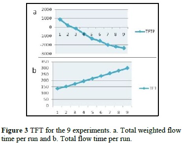
In the first 2 runs we found a positive TWFT, which indicates that Priority I jobs had a higher weight on the indicator than the Priority II jobs. From run #3, we found that Priority II jobs had a higher weight than Priority I jobs, leading the indicator to have negative values. As the number of jobs with negative priority grows, the TWFT becomes smaller and the number of jobs processed on the later date increases. The TFT increases as the number of jobs with negative priority increases (see Figure 3).

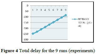
When the delay has a negative value, there is an improvement in the delivery date of a job. In the 9 runs there was always advancement. This indicator grew with the increase in priority II jobs, because they always end on later dates, closer to their deadlines, causing the gap between C_i and d_i to diminish with over the course of the runs (see figure 4).

3.4 Case 4

The case study was run without the parameter tmp, freeing the model up to schedule the activities of a job at any time, meaning that once a job starts, the model can take the time it needs to finish it.

The value of the objective function without tmp is TWFT = -5191. It takes the same value as the case study with the tmp parameter, indicating that eliminating this parameter does not affect the TWFT, since this only depends on the C_j times when the jobs finish and not in the moments when the other operations are performed. The time finding a solution is increased by 40% when the problem was solved without including tmp. The tmp parameter is especially useful when the products are perishable or when for some other reason once processing starts not much time can be spent to completion. The model with tmp presents a solution that links up much more to the operations of one single job and that cannot be performed in scattered moments in time. The use of machines is different for each of the cases.

3.5 Case 5

The tmp parameter was used, equating it to the sum of all the operation processing times. In other words, the time available between the beginning of the first operation of a job and the end of the last operation was exactly equal to the sum of the duration of its operations. Therefore, this operation is called "no wait" because no waiting times are allowed between job operations.

In the OPL operations graph, we can see how the Priority I and II jobs are scheduled in their earlier and later dates respectively without causing waits between work operations. It ensured that the first job to be scheduled is job 13 and the last is job 1. This is because job 13 has a weight of 11, the highest of all, as well as a ready time of 0, and job 1 has the lowest weight of all at -16 and a deadline of 240.

The dates for completing the jobs are maintained; what varies are the moments at which operations 1 and 2 are performed, generating a maximum clustering between the 3 operations of all jobs.

4. Conclusions

The problems of non-traditional scheduling, despite the degree of complexity in the required information and high costs (both economically and technologically), are no strangers to the reality of a company, since demand may be estimated for future periods and companies may defer the manufacturing of a product to the latest possible moment.

Tmp is a parameter which controls the degree of dispersion between activities. Hence, a large tmp allows large spans of time between the end and start of operations of the same job, while a small tmp makes operations of the same job closer to each other. Therefore the smaller the tmp of a job is, the less waiting time between the beginning of its first operation and the end of its last operation.

Since the scheduling carried out in this paper has non-traditional features, traditional performance measures, such as makespan or shop utilization, provide little information relevant for analysis. This is because when there are Priority II jobs that are completed as late as possible, the makespan will always have a value equal to the scheduling horizon, which is set by the capacity of the machines and utilization will always be the same, precisely because the C_max does not change either.

References

[1] A. Jain y S. Meeran. "A state-of-the-art review of job-shop scheduling techniques". Journal of heuristics, 1998.         [ Links ]

[2] F. Barber y M. Salido. "Introduction to constraint programming". Inteligencia Artificial, Vol 7, 2003.         [ Links ]

[3] M. Galpienso. "Un modelo de integración de técnicas de CLAUSURA y CSP de restricciones temporales: Aplicación a problemas de Scheduling". Departamento de Ciencia de la Computación e Inteligencia Artificial, Alicante, 2001.         [ Links ]

[4] D. Terekhov, M.k. Dogru, U. Ozen, J. Beck. Solving two-machine assembly scheduling problems with inventory constraints. Computers & Industrial Engineering, 2012.         [ Links ]

[5] O. Unsal, C. Oguz. Constraint programming approach to quay crane Scheduling problem. Transportation Research Part E 59, 2013.         [ Links ]

[6] R. Russell. A constraint programming approach to designing a newspaper distribution system. Int. J. Production Economics 145, 2013.         [ Links ]

[7] B. Detienne. A mixed integer linear programming approach to minimize the number of late Jobs with and without machine. European Journal of Operational Research, 2014.         [ Links ]

[8] T. Lapègue, O. Bellenguez, D. Prot. A constraint-based approach for the shift design personnel task scheduling problem with equity. Computers & Operations Research 40, 2013.         [ Links ]

[9] A. Malapert, C. Guéret, L. Martin. A constraint programming approach for a batch processing problem with non-identical job sizes. European Journal of Operational Research 221, 2012.         [ Links ]

[10] F. Brandt, R. Bauer, M. Volker, A. Cardeneo. A constraint programming based approach to a large-scale energy management problem with varied constraints. Springer Science+Business Media, 2012.         [ Links ]

[11] Y. Peng, D. Lu, Y. Chen. A Constraint Programming Method for Advanced Planning and Scheduling System with Multilevel Structured Products. Hindawi Publishing Corporation Discrete Dynamics in Nature and Society, 2014.         [ Links ]

[12] X. Wang, N. Policella, S. F. Smith, A. Oddi. Constraint-based methods for scheduling discretionary services. AI Communications 24, 2001.         [ Links ]

[13] M. Rostami, D. Moradinezhad, A. Soufipour. Improved and Competitive Algorithms for Large Scale Multiple Resource-Constrained Project-Scheduling Problems. KSCE Journal of Civil Engineering, 2014.         [ Links ]

[14] K. Limtanyakul, U. Schwiegelshohn. Improvements of constraint programming and hybrid methods for scheduling of tests on vehicle prototypes. Springer Science+Business Media, LLC, 2012.         [ Links ]

[15] J. Novas, G. Henning. Integrated scheduling of resource-constrained flexible manufacturing systems using constraint programming. Expert Systems with Applications 41, 2014.         [ Links ]

[16] Q. Ma, Z. Duan. Linear time-dependent constraints programming with MSVL. Springer Science+Business Media, LLC 2012.         [ Links ]

[17] S. Liu, C. Jung Wang. Optimizing project selection and Scheduling problems with time-dependent resource constraints. Department of Construction Engineering, National Yunlin University of Science and Technology, No. 123, 2011.         [ Links ]

[18] Y. Tang, R. Liu, Q. Sun. Schedule control model for linear projects based on linear scheduling method and constraint programming. Automation in Construction, 2014.         [ Links ]

[19] P. Bruker, B. Jurich, B. Sievers. A branch and bound algorithm for the job-shop Scheduling problem. Universitiit Osnabriick, D-49069 Osnabriick. Germany, 1992.         [ Links ]

[20] A. Ebadi, G. Moslehi. An optimal method for the preemptive job shop scheduling problem. Department of Industrial and Systems Engineering Isfahan University of Technology, 2013.         [ Links ]

[21] J. Orejuela. "Desarrollo de un modelo jerárquico de planeación de la producción en un flow shop, caso industria de concentrados". Universidad del Valle, Facultad de Ingeniería, 2008.         [ Links ]

[22] D. Gupta, P. Singla, S. Bala. N x 2 Flow Shop Scheduling Model Using Branch and Bound Technique, Set up Times are Separated from Processing Times, With Job Block Criterion and Interval of Non Availability of Machines. International Journal of Engineering and Innovative Technology (IJEIT). Volume 3, Issue 1, 2013.         [ Links ]

[23] M. Pinedo. "Scheduling Theory, Algorithms and Systems". Springe Science+Business Media, Inc. 2002.         [ Links ]

[24] M. Arangú. Modelos y Técnicas de Consistencia en Problemas de Satisfacción de Restricciones. Universidad Politécnica de Valencia, 2011.         [ Links ]

[25] M. Pinedo. Planning and Scheduling in manufacturing and services". Springer Science+Business Media, Inc, 2005.         [ Links ]

[26] F. H'Midaa, P. Lopez. Multi-site scheduling under production and transportation constraints. International Journal of Computer Integrated Manufacturing. Volume 26, Issue 3, 2013.         [ Links ]

[27] M. Relich. Fuzzy Project Scheduling Using Constraint Programming. Applied Computer Science. Volume 9, Issue 1, 2013.         [ Links ]

[28] P. Lorterapong, M. Ussavadilokrit. Construction Scheduling Using the Constraint Satisfaction Problem Method. Journal of Construction Engineering and Management. Volume 139, Issue 4, 2013.         [ Links ]

[29] Y. Rao, D. Qi, J. Li. An Improved Hierarchical Genetic Algorithm for Sheet Cutting Scheduling with Process Constraints. The Scientific World Journal, Volume 2013, Article ID 202683.         [ Links ]

[30] H. Bakker. An Introduction to the Nurse Rostering Problem. Knowledge Representation and Reasoning Seminar Report, 2013.         [ Links ]