


 English (pdf)
 Article in xml format
 Article references
 Send this article by e-mail
 Cited by SciELO
  Cited by Google
  Similars in
SciELO
Similars in
SciELO  Similars in Google
 Permalink
1. Introduction
The current society of information is facing a new challenge: Thousands of Megabytes of information are available not only in the public Internet but also in private networks. This information is used continuously, but tools for accessing and manipulation of data do not fulfill the expectations of the users, hence efficient tools are becoming a necessity.
Text classification becomes a key tool in order to deal with such amounts of information. Text classification can be used to organize document databases, filter Spam from e-mail accounts, or even to learn user’s news reading preferences. Search engines for On-line information are a kind of text classifier but they often retrieve results far from perfect.
Most of the results obtained are irrelevant, and in many cases the number of results and their ranking is far from the desired criteria. Techniques derived from Artificial Intelligence and Machine-learning theory have contributed to the improvement of such search engines, leading to better, faster and more accurate results. Kernel methods have become one reliable and robust technique well suited to deal with high dimensional problems, ideal for facing text-mining tasks. More precisely, the Support Vector Machines have been tested in such tasks leading to interesting results. These results have been obtained based on the paradigm of Inductive Inference. This paper contains the results of an application of Support Vector Machines to text classification but now based on the paradigm of Transductive Inference.
The following article is composed of the following sections: Inside the section of methodology we are to going to describe the theoretical background that is necessary to understand the research. The section 3 express experiments and results and discussion of them. Finally in section 4 we describe the different conclusions obtained from the research process.
2. Methodology
2.1 Text Classification
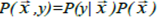
Text classification in the context of machine learning is a supervised learning approach oriented to create classifiers that automatically classify documents into a fixed number of semantic categories. Since each document can exist in either one, multiple or no category, to facilitate the task, each category is treated as a separate binary classification problem. Every document is a collection of string of characters. Such collection has to be transformed into a representation suitable for learning algorithms and classification. The Stemming tool helps to obtain such representation. The stem of a word is the canonized element of the word. That is the removal of word suffixes such as plurals, tenses, and deflections. In a given engine this stem representation is robust to spelling errors, but have the risk of returning irrelevant items. In order to obtain an attribute-value representation of a text, each word is counted within the text and its attribute is related as a feature in the vector representation.
This attribute is known as time-frequency TF ( wi,x ). The word wi exists x times in the given document. But this model is inaccurate in the sense that it assigns more weight to the word that is more frequently found in the entire document. The problem is that these words tend to be “stop words”. Stop words are words that always are present in a document such as articles “The”, ”a” and connectors such as “and”, etc. For this reason, a more adequately model is the tf-idf model (Term frequency - inverse document frequency) that counts the frequency of every word but also takes into account the frequency of the particular word in the entire document collection. The term vi,j is the weight of index term j in the document i. Such term is weighted for the tf-idf model as follows:
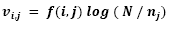
Where f(i,j) describes the term frequency of index term j in the document i. N denotes the number of documents in the entire collection and nj is the number of documents that contain the index term in their description. For the SISTA database, the model adopted was the tf-idf model [1].
The measure used in this project to evaluate the performance for text classification is Precision/Recall [2] [3]. Precision is the probability that a document predicted to be in class “+” truly belongs to this class. Recall is the probability that a document belonging to class “+” is classified into this class.
2.2 Support Vector Machines
Support vector machines were developed by Vladimir Vapnik, based on the principle of Structural Risk Minimization: To find a hypothesis h from the hypothesis space H for which one can guarantee the lowest probability of error, for a given training example. The aim is to find the classifier or discriminator function that maximizes the distance within classes, assuring the lowest probability of error. This is used to classify a set of l training examples . Each example has d features
 , for instance in a two-dimensional data input d = 2. Each of the examples has a class label with one of two values
  . In some cases, the discriminator function is constructed using a hyperplane in the space Rd. Any hyperplane can be parameterized by a vector orthogonal to the separating hyperplane
  , and a constant b (bias).

The classification function is given by the expression:

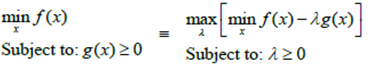
If the data is linearly separable this function will separate the data in a perfect way, and the function (2) will show the following property.

Multiple hyperplanes fulfil this requirement however the aim of the support vectors machines is to construct an optimal hyperplane that maximizes the geometric distance in the close data points, which is called the margin. (¡Error! No se encuentra el origen de la referencia.)
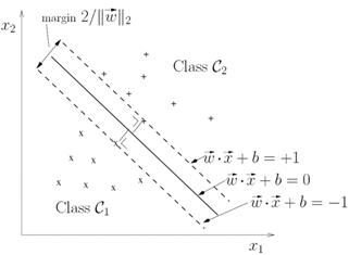
Figure 1 “Linear classification: definition of a unique separating hyperplane illustrate in a two-dimensional input space. The margin is the distance between the dashed lines”. Source [4].
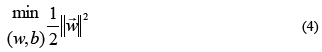
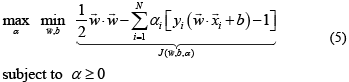
If we want to maximize the decision margin we should minimize the quadratic norm of  . The minimization of a quadratic cost function is a convex optimization problem and there are efficient numeric methods to solve it. This is a fundamental advantage of the SVM with respect to “traditional” neural networks such as the Multi-layer Perceptron whose optimal solution is only obtained by solving a non-convex optimization problem. Then optimization of the decision margin is formulated in the following way:
Subject to: 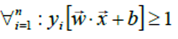
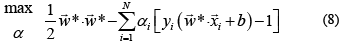
Introducing the Lagrange formulation:
Hence, writing our optimization problem in terms of Lagrange we get:
The conditions for the minimum of J in the variables  and b are:
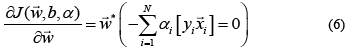
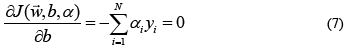
Replacing and in yields,
From (6) we obtain
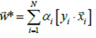
Replacing in (8) gives:
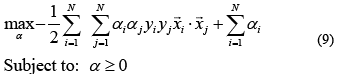
This is equivalent to
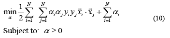
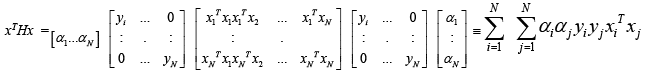
The main advantage of the Support Vector Machines is that we can solve this problem as a QP problem, the optimization problem could be written in the following form (Here in matrix notation):
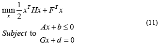
Taking into account that in our case x=( our optimization problem in terms of QP is as follows:
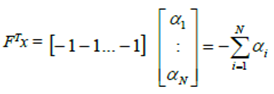
The restrictions are as follows,
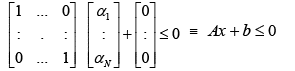
And G=[0] d=[0].
2.3 Transductive Inference
The method used to train Support Vector Machines belongs to the class of inductive inference methods. In this class of methods, particular examples are used to infer the general concept. The learner induces a decision function with a low error value on the whole distribution of the examples used during the learning phase. But in most of the situations, we don’t care about the particular function; we only need to classify a given set of examples (i.e. test set) with as few errors as possible. The transductive inference [2] uses the training examples previously labelled and the unclassified examples to generate an optimal partition and labelling of the unclassified examples, using the prior knowledge provided by the distribution of the unclassified examples.
Inductive inference generally claims for an enough amount of training data in order to determine the decision function. But for many practical uses of text classification, it is crucial to the learner to be able to generalize using little training data. Transductive inference tackles the problem of learning from small training samples [2]. This concept has been extended in recent developments by Li et al. in [3].
Some of the applications for the transductive text-classification are the following: Relevance Feedback: Used in most the customizable interfaces of the current RSS sources. After an initial query made by the user, he marks the retrieved documents as relevant or irrelevant. This composes the training set of the application. The remaining documents in the database are the test set. From this information, the learner has to classify the test set as relevant or irrelevant documents to the query. Netnews Filtering: Since there are thousands of topics available in the everyday net news. The user is interested obtaining the relevant information for his profile according to few labelled news selected during previous visits to the newsgroup. Reorganizing a document collection: Nowadays organizations are using databases of documents with classification schemas.
When one new category is created a text classifier must perform a full classification of the entire collection of documents given very few training examples. Observe that all applications have in common little training data but large test sets. More recently they has been implemented in problems with unbalanced data sets [5].
2.4 Transductive Support Vector Machines
Section 2 showed that SVMs are well suited for a learning task of the form
The learner L is given a hypothesis space H of functions  and independent identically distributed sample
Strain
of n training examples
and independent identically distributed sample
Strain
of n training examples

Where each training example consists of a document vector and a binary label. In the transductive setting, the learner is also given an i.i.d. sample Stest of k test examples.

The goal of the transductive support vector machine (TSVM) or transductive learner is to select a function hL=L(
Strain
,
Stest
) from the hypothesis space H using
Strain
and
Stest
such that the expected number of erroneous predictions on the test and the training samples is minimized. But, why not use the learning rule obtained by means of the training examples to classify the test examples? The problem arises when a small training set is used. The classifier will have a “poor” generalization due to the lack of knowledge about the distribution of points in the space X. Finding the k binary values  based on the classifier estimated with very few points will lead to disappointing results.
Unlike of the inductive setting, the transductive setting uses the location of the test examples when defining the structure. Such structure corresponds to a structure of possible hypothesis solution. Using prior knowledge about the nature of P(x,y) provides extra information to build an appropriate structure and learn more quickly. The structure is build based on the margin on both the training and the test data. For linearly separable problems, the transductive learning can be achieved by solving the following optimization problem.
OP 1 (Transductive SVM (lin. sep. case)
Minimize over 
 subject to
:
subject to
:
 and
and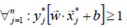
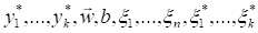
The solution of this optimization problem is not only the separating hyperplane  but also the labeling of the test set
  (Fig. 2).
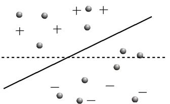
Figure 2 The maximum margin hyperplanes. Positive/negative examples are marked as +/- test examples as dot, the dashed line is the solution of the inductive SVM, the solid line shows the transductive classification. Source: Authors, modified from [2].
Most text-classification problems are linearly separable [2], but sometimes the data is non-separable by a linear function, then we can introduce slack variables  to allow some misclassification, as we do in the inductive SVM. If a training example lies on the “wrong” side of the hyperplane, the corresponding will be greater than 0. Therefore
  is an upper bound on the number of training errors [2].
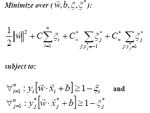
OP 2 (Transductive SVM (non sep. case)
Minimize over (
 ):
):
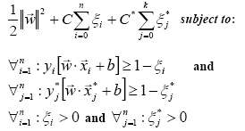
Where C and C* are the regularization parameters. They allow trading off margin size against misclassifying training examples or excluding test examples. Small values for C and C* will “tolerate” a number of training errors, while a large value for this parameters leads to a behavior similar to the linearly separable case OP1.
When we train a transductive SVM we are solving the (partially) combinatorial optimization problem OP2. For a small number of test examples, it could be done manually, trying all possible assignments  to the two classes, but it becomes intractable when the data set has more than 10 examples. The algorithm proposed by Joachims [2] is designed to handle large test sets common in text classification with more than 10.000 test examples. It found an approximate solution to the optimization problem OP2 using a form of local search.c.
The key idea of the algorithm is that it begins with a labeling of the test examples done by means of inductive SVM. Then it improves the solution by switching the labels of the test examples such that the cost function decreases. It takes the training and the test examples as input and output the labeling for the test example and a model created by means of the inductive inference.
Besides the two parameters C and C* the user can define the number of test examples (num+) assigned to the class +. This allowed a trade-off between recall-precision. The algorithm is summarized in Fig. 3. It starts with the classification of the test examples based on the inductive approach. Then it uniformly increases the influence of the test examples by increasing the cost factors and
and  up to the upper bound C* (loop 1) defined by the user. The algorithm uses an unbalanced cost of and to keep ratio num+. Loop 2 identifies two examples such that the switching of their labels leads to a decrease in the current objective function. The function solve_svm_qp refers to the quadratic program to solve the inductive problem and is presented in the following lines:
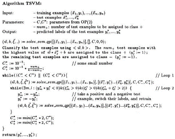
OP 3 (Inductive SVM (primal)
2.5 Why are Transductive Support Vector Machines well suited for Text-classification?
The following are special properties that every text-classification task have, such as High dimensional input space, Document Vectors are sparse and few irrelevant features [2]. Joachims argues that TSVMs are well suited and even outperform many of the traditional approaches for text-classification. Intuitively it can be explained by the fact that the transductive learning inherits most of the desirable properties of the inductive learning. TSVMs take advantage of the fact: that words occur in natural language in strong co-occurrence patterns [2]. Some words are more likely to occur together in a document than others. For example, when we ask a search engine like Google® for the words paint and sculpture it returns 25.300.000 web pages. When we ask for documents with the words paint and mathematics we get only 15.200,000 hits, although that mathematics is a more popular word in the web than sculpture. This co-occurrence is the previous knowledge that the TSVM exploit on the learning task.
3. Results
3.1 SVMLight vs. MatlabTM
Thorsten Joachims has developed SVMlight [6] that is an implementation of TSVM for the problem of pattern recognition, for the problem of regression, and for the problem of learning a ranking function. We evaluated the performance of this application against our version made in MatlabTM [7]. The MatlabTM version overcomes SVMlight in an example where from a gaussian distribution we drew 100 data points. All the data points were previously labelled into a positive and negative class (50+/50-). The data distribution is linearly separable and the learning machine was trained with 15-labeled examples as training set and 85 as test set. Joachim’s application is oriented to work with large data set with many features rather than with a two-dimensional feature vector. While the MatlabTM version reaches the perfect classification of the test examples with Precision/Recall = 100%/100% (Fig. 4), the SVMlight version working on the same set with the same parameters (RBF kernel sigma=50 ad C=0.1) gives a measurement Precision/Recall = 73.1707%/100%. Giving 96% of accuracy on the test set (11/85). There were found 11 false positives examples by means of SVMlight (Fig. 5).
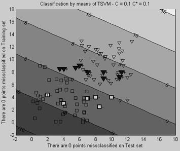
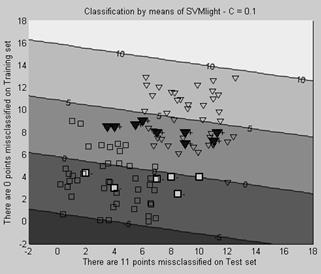
The advantage of SVMlight is its performance speed on tasks of high dimensional vectors as text classification. This characteristic will be described further.
3.2 Reuters
Given a set of 610 examples that correspond to Reuters’s articles, we have to found those that correspond to “Corporate Acquisitions”. With only 10 examples as training examples labelled 5 as positives and 5 as negatives, the TSVM must classify the remaining 600 test examples. The SVMlight algorithm is trained with this set of examples. Parallel to this we must tune certain parameters. The work with SVM demands to tune certain parameters, then some questions arise: Which kernel we can choose? What criteria for the generalization parameters C?. What amount of positives examples (num+) can we assign when we enter into loop 1 of algorithm? Demonstrations done by Joachims have shown that “non-linear SVMs do not provide any advantage for text classification using the standard kernels” [2]. So for this task, we work with a linear kernel. The best value of C depends on the data and must be determined empirically. The effective range of the C depends on the Euclidian length of the feature vectors. A good starting point of exploration is  [2].
[2].
We let SVMlight calculate C. The value of num+ regularly is the ratio of positives examples in the training data [2]. Finally, SVMlight employs only 40.42 seconds in the evaluation and creation of the model (SVM) and 1 second performing the predictions for the 600 examples. The results show 13 False Positives and 11 False Negatives. This gives us a measurement of Precision/Recall = 95.6667%/96.33%, giving 96% of accuracy on the test set (24/600). In order to evaluate the performance of the MatlabTM version of the TSVM algorithm, we test it with the Reuters task. The algorithm took 26.06 minutes computing and generating predictions for the test data. The results show 19 False Positives and 4 False Negatives. This gives us a measurement of Precision/Recall = 93.667%/98.6667%, giving 96.1667% of accuracy on the test set (23/600). This slightly improvement does not mean any significant advance in terms of results obtained. What is notoriously highlighted is the speed performance of the algorithms: 40.42 Seconds of the SVMlight against 26.06 minutes of the MatlabTM implementation. From this, it is clear that the SVMlight implementation is better suited for text-classification tasks. To automatically define the parameter C was implemented a function that computes C as the results of (avg. x*x)-1.[2][6]. With the data of the Reuters task, this function gives a value for C = 1.0033 C ≈ 1. Different tests were made in order to evaluate the accuracy of such function. Table 1 describes the results obtained when C parameter is changed.
Table 1 Reuters results with different values for the regularization parameter C. Source: Authors
| C | Precision | Recall | False P+ | False N- |
|---|---|---|---|---|
| 0,05 | 47,3333 | 99,6667 | 158 | 1 |
| 0,10 | 59,3333 | 99,6667 | 122 | 1 |
| 1,00 | 93,6667 | 98,6667 | 19 | 4 |
| 5,00 | 96,0000 | 96,6667 | 12 | 10 |
| 10,00 | 96,0000 | 96,6667 | 12 | 10 |
| 1000,00 | 0,0000 | 100,0000 | 300 | 0 |
Note that the best results are reached when the parameter C=1,00. This value corresponds to C calculated by means of the function described before. This function performs the calculation of C as Joachims suggest in his book [2].
Our MatlabTM implementation of the TSVM algorithm works adequately. The only drawback is response times. Computationally speaking the bottleneck of the TSVM algorithm is the optimization task, which has to be solved with quadratic programs (QP). We obtained worse results working in the different tests of above (toy example included) with the native QP solver of MatlabTM. For this reason, we adopt the QP solver LOQO [8]. LOQO was developed at the Princeton University NJ, and thanks to that it is pre-compile, the response times were notoriously improved. For instance, the toy example was performed using LOQO in 12.8480 seconds with an average of 0.1810 seconds per iteration.
While using the QP solver of MatlabTM it employed 3 minutes 18 seconds with an average of 12.4980 seconds per iteration. It was the main reason why we adopt LOQO as QP solver in order to perform the Text classification tasks
On Table 2 we can see also the improvements on response times. The splitting criteria allow us to go from 26 minutes employed in the original (600 examples) to only 6 minutes in the first split group with the half of the examples (300), and even better times in the other groups.
Table 2 Results obtained in the Reuters task with different amount of subsets. First column depicts the split criteria. Second and third column illustrate the measurements of Precision/Recall. The fourth column shows the times employed solving the task. The fifth column shows the times of the solve_svm_qp function. In the sixth column, the C parameter of each task is depicted. In the last column appear the number of iteration done until the upper bound C* is reached.
| No. Examples | Precision | Recall | Time Employed (Mins) | Avg. time/Iteration (Secs) | C/C* | No. Iterations |
|---|---|---|---|---|---|---|
| 600 | 93,6667 | 98,6667 | 26,0608 | 15,1812 | 1.00329 | 17 |
| 300 | 66,3333 | 96,3333 | 6,3590 | 2,6140 | 1.00000 | 17 |
| 150 | 72,3333 | 91,3333 | 2,4931 | 0,4600 | 1.00000 | 17 |
| 75 | 79,3333 | 93,6667 | 2,1069 | 0,1000 | 1.00000 | 17 |
| 50 | 87,3333 | 90,3333 | 2,2259 | 0,0300 | 1.00000 | 17 |
| 25 | 89,6667 | 90,3333 | 3,3831 | 0,0100 | 1.00000 | 17 |
The improvements in the response times can be explained due to the fact that we are performing less computation in the construction of the linear Kernel  this also involves the computation of the Hessian in the optimization problem (OP3).
Splitting the test examples we can obtain better results in response times, but it means also a sacrifice of precision/recall in the entire task. It can be overcome if we divide considerably the test set. So we have to find the trade-off between precision/recall and response time.
3.3 SISTA Database
The SISTA database corresponds to the model that describes the ESAT library. This database has been built by the text mining group of SISTA (Research division of the department of Electrical Engineering (ESAT) at the KU Leuven) [1]. This model includes a feature vector representation of each book as well as various database tables that allow the research process in text-mining.
In order to apply the TSVM algorithm to the SISTA library, the entire collections of books (1429 Titles) are loaded to the MatlabTM environment. In the first test, we worked with the table ix_library_v1 that have the indexed data including stop words [1].
For the creation of the training examples 10 records were labelled as positives, and they were selected among the books that have the word “Control” in his title. On the other hand, 11 examples that have the word “Learning” were selected as negatives examples. We then evaluated the TSVM algorithm, looking for the classification of the 1408 test examples based solely on the 21 examples of training and the position of the test examples.
The TSVM algorithm took 3 hours (201.99 minutes) in solving the classification task. This process was run on a computer with Intel Core 2 Duo processor of 2 GHz with 2 GB of RAM. Which make it unreasonable to implement in a Web search engine, where the response times are expected to be minimum.
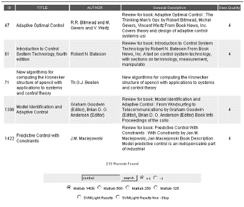
In order to verify the results, we integrate the tool in the intelligent interface web engine. In such interface, we typed the word “Control” trying to find the books in the test examples that have this word in his title. 213 titles are retrieved (Fig. 5).
Evaluating the results of the classifier, the web interface allows searching within the positive classified examples. We performed the same search of above and 204 of the total 213 books were retrieved.
Apparently, 9 books were labelled as false negatives for the classifier. Now, analyzing this book titles we see that the field of “Description Quality” not has any information for 7 of the 9 titles.
A missing quality label means that a review was not found on the internet by the web crawler or because Amazon.com did not have a review available for the book (this is the case for 207 books, e.g. because it is a Dutch book) [1].
The other two examples have been scored with “4” meaning that the review is no reliable (see above); in fact, one of the books is in Dutch what excludes it of any possible classification. The remaining book has the title: “Evolutionary Learning Algorithms for Neural Adaptive Control” Indeed this book fall more in the negative class where 10 books with the topic “learning” were selected as training examples.
These results show interesting clusters found within the SISTA library. The above experiment proves that the algorithm performs good classification of the books with this small quantity of examples. The only drawback still being the response time that continues making impractical the application.
Table 3 shows different test made in order to overcome the response time problem. As in the Reuter experiment, the test set is split into different groups. The subset or groups are now of 500, 250 and 125. Note the improvements in times of response (“Time employed”,”Avg time/Block” and “Avg time/iteration” columns).
Table 1 . Split strategy for SISTA database task.
| No. Example | Positives | Negatives | Diff W.R.T. 1408 | Time Employed (Mins) | Avg. time/Block (Secs) | Avg time/ Iteration (Secs) | C/C* | No. Iterations |
|---|---|---|---|---|---|---|---|---|
| 1408 | 704 | 704 | 0 | 201,99 | 201,99 | 20,51 | 1 | 17 |
| 500 | 642 | 766 | 288 | 2,3675 | 50,93 | 0,95 | 1 | 17 |
| 250 | 680 | 728 | 342 | 0,55 | 5,44 | 0,155 | 1 | 17 |
| 125 | 768 | 640 | 404 | 0,707 | 3,68 | 0,054 | 1 | 17 |
Outstanding changes are depicted in the results: the amount of examples that diverge with the original classification are counting in the “Diff W.R.T. 1408” column. On it we can see that the smaller the group of examples the greatest the difference in the results. The number of iterations as C parameters does not change in any of the experiences. It is logical: since the upper bound of the loop 2 of the algorithm (that controls the number of iterations) is given for C*.
The same example was run in the SVMlight [6]. The results show 670 examples classified as positives.
The interesting thing here is that there are 50 examples differently classified by this software. Searching in the classified positives examples for books with the word “Control” in his title, the retrieval results were different. This software only classified 139 examples with the word “Control” as positives examples.
The main advantage of this application is that it takes only 10 minutes in order to solve the problem. But still being impractical to implement in a web search engine. Further analysis on this data becomes difficult because we do not have model examples of classification.
A copy of the code can be found in [9].
4. Conclusions
When we look back at the initial goal of the project, we think we can say that we succeeded in meeting the main requirement. We have implemented a kernel classifier based on the transductive inference methodology. We were able to implement the transductive induction by means of the TSVM algorithm of Joachims [2].
The fact of being able to classify all a set with few examples of training makes of this algorithm a solution for the huge task of organising and index the huge amounts of data available in the actual information society.
Thanks to the different types of examples with which we could evaluate the TSVM algorithm (see Fig. 3), we can say that it fulfills the expectations and completes the classification tasks with relative accuracy.
One of the main advantages of TSVM is that it does not have to tune many parameters as traditional SVM. The kernel selection is straightforward because “non-linear SVMs do not provides any advantage for text classification using the standard kernels” [2]. The parameter of regularization “C” is calculated heuristically and taking into account the data of the particular task. This strategy proved to be effective. Finally, the number of examples assigned to the positive class (loop 1of the algorithm) in most of the cases corresponds to the half of the test data.
The only drawback found in the TSVM algorithm was the response time. In order to solve it, the splitting strategy was implemented. This solution solves the problem of the response time but sacrifices precision/recall. This is logical since the algorithm evaluates the totality of the test examples in order to define the final optimal classifier. If we train each of the TSVM on a smaller test set, we are not exploiting the 'Transductiveness' to the full extent. This reflects in a reduced performance.
Working with the SISTA database, the algorithm completed the task after 3 hours, which made impractical the integration done in the already developed Intelligent Interface Web Engine [1] from the SISTA group. A search engine on Internet demand reasonable response times and a delay of 3 hours is unthinkable in a web system. Even for the most patient of the users.
We recommend for further implementations try to use a parallelized strategy, in order to optimize the multiples core that the Processors technology of nowadays offers. Once the algorithm is parallelized, it can also be evaluated in platforms as MathWorks Cloud which is powered by Amazon EC2 ® [10].

