


 English (pdf)
 Article in xml format
 Article references
 Send this article by e-mail
 Cited by SciELO
  Cited by Google
  Similars in
SciELO
Similars in
SciELO  Similars in Google
 Permalink
1. Introduction
According to the standard cosmological model, the recession of galaxies at large distance scales (the Hubble flow) is expected to exhibit motion subject to Hubble's law. This condition follows from the anisotropy and homogeneity of space, which is expressed in the cosmological principle. Observations of the Cosmic Microwave Background (CMB) and matter distribution in large scale surveys have been generally consistent with homogeneity and isotropy; however, recent analysis of CMB data has identified the presence of anisotropies, which are potentially intrinsic [1].
This paper explores the use the Hubble flow as a probe of intrinsic anisotropies. Looking at systematic differences in recession velocities in opposite directions provides a direct method to identify intrinsic anisotropies. A challenge, however, is to be able to discriminate between intrinsic anisotropies and anisotropies generated by large scale bulk motions. At non-cosmological scales, galaxy velocities are affected by proper motions and deviations from a smooth Hubble flow due to voids and regions of mass over-density. McClure and Dyer [2] used the galaxy sample from the Hubble Space Telescope Extragalactic Distance Scale Key Project (HST-KP) to map out variations in the Universe's expansion.
Their method relies on constructing a map of a continuous scalar field based on Gaussian smoothing the available H0 discrete measurements segregated at their various locations on the celestial sphere. The paper reported the detection of a 9 km s-1 Mpc-1 anisotropy in the Hubble parameter ( H0 ), however, the results are highly dependent on the strength of the smoothing that is applied to the data. Furthermore, no attempt was made to incorporate the measurement errors in their analysis.
We developed a different approach to detect anisotropies in the Hubble flow that, in contrast to McClure and Dyer, take into account observational uncertainties and is not dependent on data preparation procedures [3]. The approach consists of a Least-Squares (LS) fit of a spherical harmonic function to the H0 data (with errors). We have applied the LS analysis to a galaxy sample that includes a larger and more recent (and more accurate) set of distance and redshift measurements. Due to the limited sample size, only the dipole, ℓ = 2, term of the harmonic expansion is used. A known drawback associated with harmonic analysis is that when the data is fragmented and the harmonic series is truncated, there is potential risk for aliasing harmonic terms resulting in power leakage from higher to lower harmonics.
Due to power leakage, the harmonic coefficients from the fit may be biased. To correct these biases, a Monte Carlo simulation is used in order to compute the factor by which the dipole amplitude of a known input H0 field is affected by the fit. Key to the reliability of the analysis is to use a realistic estimation of the errors associated with the measurements of H0 in the fit. As with any x2 minimization LS fit, use of incorrect measurement errors in the computations could yield local minima that are far from the actual minima. The analysis here uses the directly measured data (i.e. distance and redshift, not H0 ), so that measurement errors can be properly incorporated. Section 2 presents the analysis approach and the treatment of measurement uncertainty; Section 3 the analysis and results and Section 4 conclusions.
2. Measuring Anisotropies in H0
Consider a galaxy catalogue with measurements of redshift (z) and redshift-independent distances (d). Each galaxy in the catalogue contributes with a pair of measurements {z i ,d i } and respective measurement errors. For each {zi,di} pair, a value of H0 is computed, H0,i = vi/di. The set of H0,i values form a discrete scalar field.
Define the function H(8,p) in terms of a dipole vector D:

The unit vector n is the direction of observation. The vector D with Cartesian components Dx,Dy and Dz represents the direction along which the scalar field H(θ,φ) exhibits maximal variation at 180° angular scale. The norm of D is the amplitude of the anisotropy. The LS fit finds the coefficients {Dx, Dy, Dz} that minimize the X2:
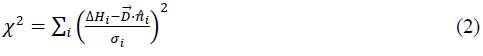
Where, al is the error associated with Hy, and

Ĥ0 is the average of all H0 measurements.
2.1 Galaxy sample
For this study, the galaxy compilation of Freedman and Madore [4] was used. Distances and redshifts were obtained from the NASA/IPAC Extragalactic Database (NED) [ned]. Galaxies with distances < 45 Mpc were discarded in order to remove proper motion effects. Recession velocity was computed from the redshift measurements and transformed from the heliocentric to the CMB frame. Galaxies with Vcmb < 700 km s-1 were discarded.
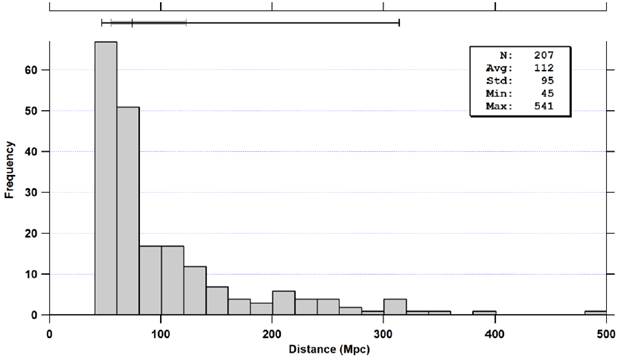
The Hubble parameter of each galaxy was computed. H 0 outliers were removed: H 0 > 94 and H 0 < 46. H 0 units used in this paper are km s-1 Mpc-1 and will not be explicitly given henceforth. After all the cuts to the data, a sample of 207 galaxies was left in the analysis. The sample spans a distance range between 45 and 500 Mpc (Fig. 1), with the bulk of measurements in the 45 to 100 Mpc range. Most of the galaxies in the sample have distance measurements that use different distance determination methods. For the 45-100 Mpc distance range the methods most used in the sample are Fundamental Plane, Faber-Jackson, SNII, SNIa, Tully-Fisher, and D-Sigma.
2.2 Error Modeling
Entries in the NASA/IPAC catalogue are obtained from publications. Unfortunately the astronomical community does not have a unified and consistent manner to report galactic distance errors. Distance errors are affected by a number of factors related to the accuracy of photometric measurements and the zero point calibration of the distance scale. For a galaxy in the catalogue that has N measurements, a reasonable approach to assess the error of its distance is to compute the standard deviation of the mean(=StDev/ N ). If the N measurements are independent and combine different distance calibrator methods then this estimate is a good representation of the total measurement error.
If all the N measurements use the same distance calibrator, then this error estimate would not reflect distance calibration errors. A practical way to account for measurement and calibration errors is to use the standard deviation of the mean in combination with a nominal calibration error (5 Mpc) added in quadrature. For galaxies in the catalogue with N < 3 an error of 0.13 d (d = distance) was used.
This relative distance error of 13% is the best fit to the distance errors in the redshift independent distance measurements of the NED-D compilation [5]. The dominant error in the computation of H0 is distance. For estimation of velocity errors, a similar approach as with distance is followed using a nominal systematic error of 100 km s-1.
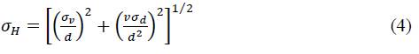
The error going into the X2 (Eq. 2) is the error for each i-th galaxy in the catalogue, computed as follows:
3. Analysis and Results
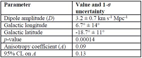
The fit converges to a solution with a dipole of amplitude 3.2. Table 1 shows a summary of the results. The 1-σ uncertainty in fit parameters is estimated by means of Monte Carlo runs where 50000 simulated galaxy catalogues were generated, using the same locations of the galaxies in the analysis and generating random distance and speed Gaussian errors according to the respective errors for each galaxy in the catalogue.
The amplitude of the dipole (D) has been multiplied by a bias correction factor of 1.03 to adjust for power leak from higher harmonics, as mentioned in the introduction. This factor was found by comparing the average of the dipole amplitudes from the Monte Carlo run with the true value used in the Monte Carlo.
The p-value is the probability that a value of D equal or greater than 3.2 would be obtained by chance (due to just random errors in distance and redshift) if in reality there were no dipole anisotropy (Dtrue = 0). The p-value was computed with a separate Monte Carlo run where the input true dipole of the simulation is set to Dtrue = 0. The anisotropy coefficient A is defined as A = 2D/Ĥ 0 .
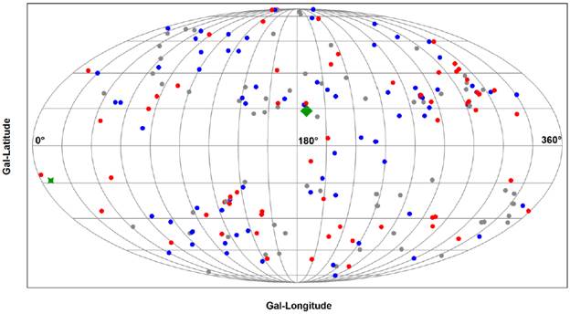
Figure 2 shows an all-sky map Mollewide projection (galactic coordinates) with the locations of the galaxies in the sample. The color code indicates deviation from average H0 value: H0 < 67 (blue), 67 < H0 < 73 (gray), H0 > 73 (red). Also indicated are the location of the dipole maximum (green star) and minimum (green diamond). An inspection by eye indicates that, as expected, there are more red than blue dots around the region centered on the dipole maximum and more blue than red dots around the minimum of the dipole.
An independent verification of the presence of systematic anisotropy in the data was obtained by means of a straightforward hypothesis testing exercise where two values of H0, representing the values at the opposite directions of the dipole vector, were compared in a statistical sense. Samples of galaxies distributed in two groups were formed by defining two cones of 50° aperture aligned in the direction of vector D and in the opposite direction. Two values of H0 (H0,pos and H0 ,neg) were computed using all of the galaxies that fall inside each of the cones respectively.
The results are: H0,pos = 73.2 and H0,neg = 67.3, a difference of 5.9 consistent with the dipole peak-to-peak difference of 6.2. Fig. 3 shows the distributions. A t-Test comparing these two values indicates that the observed difference has a statistical strength of 2.7σ. The t-Test has a p-value = 0.01, which means that the null hypothesis (that there is no anisotropy) can be rejected with high confidence. Note that the t-Test does not depend on the estimated galaxy distance errors, instead it uses the variance intrinsic in the H0 values.
It should be noted that this result may be due to galaxy sampling and systematic error- induced bias introduced due to all the different extragalactic redshift-independent distance measurement methods included in NED-D.
3. Conclusions
A dipole anisotropy of 6.4 ± 1.4 km s-1 Mpc-1 in the expansion rate has been detected. This result is consistent with the anisotropy reported by McClure and Dyer. The t-Test together with the Monte Carlo estimated low (false-positive) probability of obtaining a dipole of 3.2 just by chance, provides solid justification for the reported anisotropy.
Considering the range of distances explored (45 - 100 Mpc) it is still possible that the observed anisotropy is the result of bulk velocity flows. The direction of the dipole maximum is within 2-σ of the direction of voids (ℓ = 330°, b = -30°) that have been proposed to explain the CMB quadruple and octupole alignment [6].
However, a better understanding of error behavior, especially for distance measurements that do not report any uncertainties [7]. With the availability of new high redshift surveys [8] it will be possible to extend this analysis to cosmological distances in order to probe intrinsic Hubble flow asymmetries or in general more precise Hubble constant measurements [9] [10].
This work demonstrated that the approach of using H0 as a probe for space anisotropies can be robust and direct. The presence of anisotropies in H0 also highlights the need to take these anisotropies into account for precision measurements of H0 and in general of extragalactic distance measurements [11] in the post HST-KP epoch where goals of 1% accuracy have been set.

