


 Inglês (pdf)
 Artigo em XML
 Referências do artigo
 Enviar este artigo por email
 Citado por SciELO
  Citado por Google
  Similares em
SciELO
Similares em
SciELO  Similares em Google
 Permalink
I. INTRODUCTION
SEISMIC imaging as part of exploration seismology is focused on building physical properties images to gain better insights of earth subsurface; it is founded on how seismic waves can collect information of those properties while traveling into determined medium, and this feature is greatly exploited in several imaging reconstruction methods [1],[2] and its applications [3]. Due to the aforementioned, simulation of wave propagation has become a necessity; however, implementation of numerical modeling is widely known to be a costly computational method mainly because of the amount of information to process; furthermore, this cost is increased if complex subsurface models are considered as it is the case of the elastic model.
Due to the high consumption of computing resources, the implementation of numerical elastic modeling is still a challenge to deal with in terms of computational performance. Nevertheless, development in graphical processing units (GPU) [4] and the emergence of new programming paradigms as heterogeneous computing and High-Performance Computing (HPC) [5],[6] have let to tackle this problem by reducing time elapse, memory consumption, and other metrics; even though the necessity of improving performance is still present.
Based on the previously mentioned, finding new strategies to implement numerical elastic modeling, which explores new programming techniques, technological developments, and hardware equipment, is highly appreciated. This study presents a comparison of two elastic wave modeling algorithms running in GPU, which exploit three different features of hardware programming such as kernel launching layout, CPML memory allocation management, and CPU-GPU memory transference. In the end, an evaluation between both algorithms is performed using metrics like execution time and memory consumption to determine which one has better performance.
II. METHODS
A. A. Elastic wave modeling
Numerical wave modeling is considered a powerful tool for simulating how seismic waves travel over different subsurface layers in the earth. Elastic wave modeling considers that the earth could be modeled by three parameters named λ, μ, and ρ; those parameters are related to each other by elastic wave propagation set of equations presented by Virieux in the P-Sv form [7] in equations Eq (1), Eq (2), Eq (3), Eq (4), Eq (5).
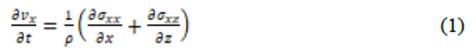


Where x and z are coordinates on the plane, v x and v z are velocity components, σ xx , σ xz, and σ zz are the stresses, and finally, φ correspond to the seismic source which generates the wave to be propagated. Simulation of the source is performed commonly using a Ricker wavelet given by the expression Eq (6).

B. B. CPML implementation
When implementing numerical modeling, an undesired behavior of wave reflection is found at the boundaries of the model. To avoid this issue is necessary to establish some energy-absorbing artificial zones near the boundaries and prevent reflections from appearing.
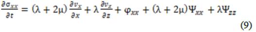
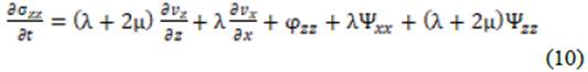
There are several methods to perform this task; among them, Convolutional Perfectly Matched Layers (CPML) [8] is widely used because it has proved to be very effective in reducing energy from seismic waves compared with other classic options. Basically, CPML method adds auxiliary variables to the modeling expressions set presented, as shown in equations Eq (7), Eq (8), Eq (9), Eq (10), and Eq (11).


Those auxiliary variables are updated following expressions in Eq (12) and Eq (13)


Where i and k are x or z coordinates depending on which variable is working, a and b represent attenuation coefficients given by the method.
C. C. Discretization
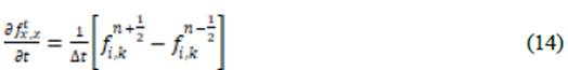
There are several numerical methods for solving the propagation equations; among them, finite differences (FD) are widely used because of their easiness of implementation. A decision to use the second order in time and fourth order in space option was made since it allows to achieve an adequate balance for numerical efficiency and small truncation error. Equations Eq (14), Eq (15), and Eq (16) represent discretization expressions for differential operators, which are applied over propagation equations.
The discretization procedure generates a grid distribution of the model where all physical dimensions are adapted into memory spaces that will contain information related to elastic parameters; in this grid, the length and depth dimensions are turned into memory locations N x × N z depending on step sizes Δx and Δz; it is common for avoiding anisotropic effects in modeling to choose Δx = Δz = Δh; discretization result is shown in Fig. 1a. To properly implement elastic modeling is necessary to use a staggered-grid scheme [9] since velocity fields update depend on stress fields located in other position as shown in Fig. 1b
D. D. Thread/Block launching layout on GPU for elastic wave modeling
Nvidia Graphic Processing Units (GPU) contains Streaming Multiprocessors (SM) as the main component for launching Threads and groups of threads known as Blocks, SM schedules necessary resources to run Kernels containing the code to be parallelized through the application of Threads/Blocks layouts [6],[10]; in the case of elastic wave modeling the parallel code comprise the propagation equations already presented. Once the grid from discretization is created is possible to allocate GPU memory (that could be seen as a matrix) and design launching layouts to properly run kernels and implement modeling.
When implementing a specific layout over a matrix, usually the first approach considers using one thread to perform calculations per every memory space allocated since is the simplest and easiest option; this distribution leads to a 1D layout where there is one big block containing all threads processing completely the memory space giving a total number of threads per block of N x × N z . Even though the mentioned 1D layout is the first option, it is not a practical implementation since GPU hardware architecture limits block sizes to contain a maximum of 1024 threads per block, which directly limits the model size to be processed with this layout.
Another design considers the allocation of threads to correspond with N x memory spaces, and the number of blocks will be bound to N z value, which represents the rows in a matrix configuration; this configuration still keeps the 1D fashion introduced in the previous example, but in this case, the number of blocks utilized is incremented, this design is presented in Fig. 2a. This layout improves over the previous, allowing to work with bigger size models but still is limited for block size limit since, in this case, a row with more than 1024 components could not be adequately processed.
In addition to previously mentioned of resource allocation in Nvidia hardware when launching layouts, it is important to mention that GPU architecture considers groups of 32 threads internally as a structure called warp; when launching a Kernel all threads allocated in the selected layout are divided to adjust them into the warp size and later some of those warps are launched concurrently.
The number of warps available to run simultaneously depends on the distribution of registers and shared memory made when one layout is established; however, this resource scheduling is not directly controlled by the programmer because it is performed automatically by GPU. Due to this lack of control by the programmer, the appropriate layout design is important for better use of GPU resources, but there are no specific instructions to follow when designing launching layouts. Therefore, it becomes an empiric procedure highly depending on the application and hardware availability.
The number of warps available to run simultaneously depends on the distribution of registers and shared memory made when one layout is established, however, this resource scheduling is not directly controlled by the programmer because it is performed automatically by GPU. Due to this lack of control by the programmer, the appropriate layout design is important for better use of GPU resources, but there are no specific instructions to follow when designing launching layouts. Therefore, it becomes an empiric procedure highly depending on the application and hardware availability.
Despite the aforementioned, Nvidia has given some suggestions [11] that could help in layout design; among them, they recommend to keep the number of threads per block a multiple of warp size, avoidance of small block sizes, and carry the number of blocks to a much greater number than SMs. By taking those recommendations, it is possible to propose a new layout as depicted in Fig. 2b
This distribution is achieved by dividing the discretization matrix into smaller 2D matrixes of the specific size to cover the space of the bigger, those smaller matrixes will correspond to the blocks in the layout, and each of these blocks will have a 2D thread distribution internally. In this way, it is possible to work with a greater quantity of blocks while keeping threads per block as multiple of warp size; this layout also lets dealing with bigger model sizes easily with no major changes.
There are many possibilities for selecting a 2D layout suitable for a determined model, a useful suggestion given by Nvidia best practices guidelines [11] would be to execute kernels based on a block size of 128 or 256 threads.
E. E. Common and reduced memory CPML memory allocation strategies
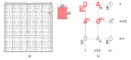
When implementing numerical modeling is crucial the definition of absorbing zones for CPML processing; those areas of fixed thickness and length are depicted in Fig. 3a. In the image is clearly differentiated two big areas named Regular and CPML zones, in the first, seismic waves travel unaltered while in the latter wave energy is reduced as you go deeper in that area.
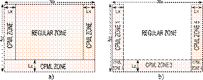
Fig. 3 CPML zones distribution and memory allocation: a) common CPML allocation strategy, b) CPML reduced memory strategy
Each CPML zone has a specific thickness L x or L z that extends to cover fully the corresponding dimension N z or N x ; when implementing over GPU those zones must have their own memory space, apart from that used for updating velocity and stress fields, where specific CPML calculations are performed.
It is common to find CPML implementations in elastic wave modeling that allocate memory spaces of N x × N z bytes looking to keep the easiness in code programming but sacrificing valuable GPU memory resources.
When using a common scheme, the amount of GPU resources invested in operations is greater since on every iteration a CPML kernel is executed, it covers completely (colored in Fig. 3a) the model memory space allocated including regular zone where is supposed not to be performed any CPML instruction. However, indexing memory locations, jumping over indexes, and internal instructions come about, which lead to GPU memory and processing threads to be misused, in addition, this inefficient behavior could be worsened if bigger size models are considered.
Another alternative to deal with CPML processing considers 5 CPML zones with reduced memory allocation to keep better control on memory resources and code execution. In addition, Kernels for CPML operations avoid accessing the regular zone, as shown in Fig. 3b.
Unlike the common implementation, the new proposed distribution considers 2 independent memory allocation zones of size L x × (N z - L z ) bytes, another 2 of (L x × L z ) bytes, finally, 1 area of (N x - 2L x ) × L z bytes; using this scheme assures that total memory used in GPU decreases even in cases where model sizes are bigger since allocations formulas only rely on 1 dimension from the model while maintaining constant the other which in most cases is a low value L x or L z .
It is important to mention that the amount of GPU resources saved in the new scheme decrease when model size dimensions are diminished, leading at some point to a virtual match in performance for both implementations of CPML processing, however in a practical application of elastic modeling where is common finding survey areas covering several kilometers of length and depth this strategy could be useful for more efficient resources management in the GPU.
F. F. CPU-GPU memory management for wavefield cube storage
According to Nvidia Best practices guidelines [11], GPU memory optimization is the key area to develop when algorithm performance is looked for; this is particularly applied in elastic wave modeling where high-performance levels are expected, especially in execution time and memory consumption because this method is usually used as the first stage in more complex procedures as inversion [2],[12] and migration [13].
Programming over GPU involves the implementation of heterogeneous computing [5] paradigm was basically a CPU act as the controller for execution flow of the program and GPU perform necessary heavyweight operations; each hardware device has its own memory space and one algorithm running under this paradigm necessarily will share information between those spaces for proper execution.
Nvidia GPU architecture based its kernel execution procedure over a memory hierarchy, which includes several memory types; among them, the registers, shared and global spaces are worth to be considered since they are the most commonly used in general applications. Registers and shared memory are the fastest memory in GPU, but those resources are limited to some Kilobytes, whereas global memory (VRAM) is slower, but there are much more available for use, which makes it ideal for dealing with big size wavefield cubes from modeling.
When executing elastic wave modeling is important to save velocity and stress fields updated and later perform the creation of a wavefield cube with those fields. To achieve that, Fig. 4 presents one approach where GPU updates one wavefield and transfers it to CPU system memory on every iteration. In this approach, elastic modeling is performed by executing Kernels that update wavefield iteratively; once the field is updated, a data transference carries that field from GPU global memory to CPU over PCI-e bus; when the wavefield reaches the system memory, it is saved, and execution of next iteration for wavefield update in GPU is allowed.
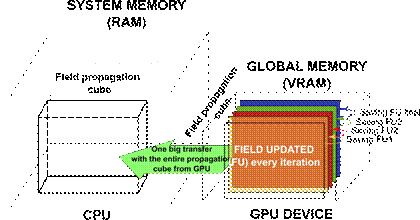
The main drawback in this strategy is associated with the reduced bandwidth available in the PCI-e x16 channel giving a maximum of 16GB/s whereas the VRAM-GPU bandwidth could peak a maximum of 128GB/s (in a Nvidia Turing Gtx 1650 card). In addition to bandwidth, the overhead due to GPU-CPU transfers could impact the execution time of wave modeling.
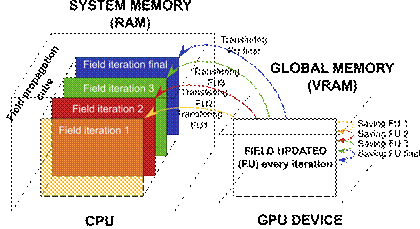
Another strategy for wavefield cube storage is depicted in Fig. 5; in this case, the GPU updates the wavefield, but this time is kept in global memory and saved on it, creating the cube; once the propagation is finished, a full cube transference is performed to CPU. This strategy overcomes most disadvantages of the previous scheme by exploiting the higher bandwidth on GPU transfers to speed up the execution of kernels and construction of propagation cube; likewise, it performs only one big transfer between GPU-CPU memory spaces which could reduce impact in execution time due to overhead.
III. RESULTS
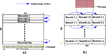
Proposed tests intent to quantify the impact of GPU launching layout schemes, GPU memory management, and data transference when an elastic modeling algorithm is executed. Two different algorithms named Algorithm 1 and Algorithm 2 were developed to execute elastic modeling; the flowchart in Fig. 6 depicts the general steps included in the programming, differences in execution come about when choosing CPML memory scheme (number 1), thread/block layout (number 2) and storage of wavefield cube (number 3).
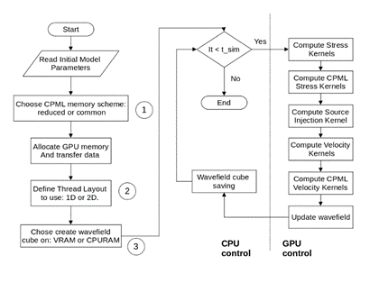
Fig. 6 Flowchart for implementation of elastic modeling in a heterogeneous system highlighting specific locations where both strategies tested differ.
Algorithm 1 implements a 2D thread/block layout for launching GPU Kernels, it also uses the CPML reduced memory allocation strategy, and it manages wavefield creation of v x field in VRAM in the GPU, on the other side; Algorithm 2 considers a 2D thread/block layout initially and later is changed to 1D layout, it includes common CPML memory allocation and wavefield construction for v x field is performed using RAM memory of the CPU.
Wave propagation implemented uses 2nd order in time and 4th in space finite differences option, space steps of Δx = Δz = 5m and a time step of Δt = 1ms, an isotropic and homogeneous medium with two planar layers with velocities V p = 3000 m/s and V p = 1500 m/s respectively, the two layers shared other parameters as V s = 1730 m/s, ρ = 2500 Kg/m3; the source is simulated by Ricker wavelet with a central frequency of 15Hz. Hardware specifications include a standalone station with a CPU Ryzen 5 3550H, 8GB of RAM; it contains a GPU GTX 1650 from Nvidia with 4GB of Video RAM; the system runs under Debian OS, and the language used for programming is CUDA C.
Fig. 7 shows four snapshots of elastic wave modeling implemented over an area of 2560 m × 1280 m, which corresponds to a wavefield of 512 × 256 points with selected discretization.
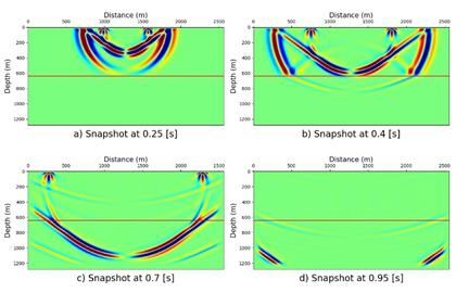
Fig. 7 Elastic wave modeling snapshots in isotropic medium with two layers. a) t = 0.25 s, b) t = 0.4 s, c) t = 0.7 s, d) t = 0.95 s.
Table I summarizes the results for execution times of each algorithm implemented (Alg 1 and Alg 2) in three tests where elastic modeling was performed at three simulations times using three different model grids. In this case, both codes use 2D layout in order to isolate the impact of memory management and data transference from Kernel launching scheme. Measurements show that Algorithm 1 improves execution time over algorithm 2, ranging from a minimum of 8.9% to 18.1%; there is also a continuous enhancement in execution time when rising both simulation time and model size; however, a specially pronounced improvement trend is detected when model size is incremented.
TABLE I EXECUTION TIMES FOR ALGORITHMS 1 AND 2 CONSIDERING 3 DIFFERENT MODEL SIZES AND 3 SIMULATION TIMES, BOTH ALGORITHMS USE 2D LAYOUT
| Simulation time (s) | Model size (points) | |||
|---|---|---|---|---|
| 256 × 256 | 512 × 256 | 512 × 512 | ||
| t sim = 1 s | Alg 1 (s) | 1.01 | 1.48 | 2.25 |
| Alg 2 (s) | 1.10 | 1.64 | 2.56 | |
| Diff (%) | 8.9 | 10.8 | 13.7 | |
| t sim = 1.5 s | Alg 1 (s) | 1.37 | 2.00 | 3.24 |
| Alg 2 (s) | 1.50 | 2.30 | 3.72 | |
| Diff (%) | 9.4 | 15.0 | 14.8 | |
| t sim = 2 s | Alg 1 (s) | 1.69 | 2.57 | 4.14 |
| Alg 2 (s) | 1.86 | 2.98 | 4.89 | |
| Diff (%) | 10.0 | 15.9 | 18.1 | |
Table II collects the same information as in table I, and similar tests were performed; however, in this case, algorithm 2 implements a 1D layout. The idea at this point is to measure execution times in codes which use not only different CPML memory management strategy but also different launching schemes. Results show vast gains in time of algorithm 1 over 2 varying from 42.5% climbing to 88.4%; likewise, there is an improvement trend going upwards with increments in simulation time and model size. It is important to mention that major gains in execution time were obtained with bigger model sizes tested according to data from both tables I and II.
TABLE II EXECUTION TIMES FOR ALGORITHMS 1 AND 2 CONSIDERING 3 DIFFERENT MODEL SIZES AND 3 SIMULATION TIMES, ALGORITHM 1 IMPLEMENTS 2D LAYOUT WHEREAS ALGORITHM 2 IMPLEMENTS 1D LAYOUT
| Simulation time (s) | Model size (points) | |||
|---|---|---|---|---|
| 256 × 256 | 512 × 256 | 512 × 512 | ||
| t sim = 1 s | Alg 1 (s) | 1.01 | 1.48 | 2.25 |
| Alg 2 (s) | 1.44 | 2.22 | 4.04 | |
| Diff (%) | 42.5 | 50.0 | 79.5 | |
| t sim = 1.5 s | Alg 1 (s) | 1.37 | 2.00 | 3.24 |
| Alg 2 (s) | 2.01 | 3.17 | 5.83 | |
| Diff (%) | 46.7 | 58.5 | 79.9 | |
| t sim = 2 s | Alg 1 (s) | 1.69 | 2.57 | 4.14 |
| Alg 2 (s) | 2.52 | 4.29 | 7.83 | |
| Diff (%) | 49.1 | 66.9 | 88.4 | |
Table III includes data related to GPU memory used for each algorithm over different model sizes; the Diff column shows how much more memory algorithm 2 used compared with algorithm 1. This value ranges from 2 to 30MB. Column Proportion/model size presents how many times additional memory used in algorithm 2 is above the memory necessary for saving a model in GPU. Figures on those columns allow us to identify a rising trend in memory consumption of algorithm 2 over 1 due to the strong relation between memory used and model dimensions N x - N z for CPML calculation in algorithm 2. This relation is reduced when implementing CPML reduced memory strategy and thus, the impact on the memory used.
TABLE III VRAM USE FOR ALGORITHM 1 AND 2 CONSIDERING 5 DIFFERENT MODEL SIZES AND A SIMULATION TIME OF 1.5 S
| Model size (points) | t sim = 1.5 s | ||||
|---|---|---|---|---|---|
| Alg1 (MB) | Alg2 (MB) | Diff (MB) | Model Size (MB) | Proportion/ Model size | |
| 256 × 256 | 435 | 437 | 2 | 0.250 | 8.0 |
| 512 × 256 | 815 | 819 | 4 | 0.500 | 8.0 |
| 512 × 512 | 1577 | 1583 | 6 | 1.000 | 6.0 |
| 768 × 512 | 2345 | 2361 | 16 | 1.500 | 10.6 |
| 768 × 768 | 3515 | 3545 | 30 | 2.250 | 13.3 |
IV. CONCLUSIONS
The results show that one algorithm using only CPML reduced memory strategy together with wavefield cube creation in GPU improves execution time by a maximum of 18.1% in tests. There also exists a continuous enhancement trend with model size increments and higher times of simulation. If a 2D launching layout is added to the strategy, the figures are increased, ranging from a minimum of 42.5% to a peak of 88.4%. In all cases, major gains were obtained when working with the bigger model sizes for all times of simulation. From data, it is noticeable the tremendous influence that Kernel launching layout has over execution time compared with CPML memory management; however, the combined effect is outstanding.
Bigger memory gains for algorithm 1 over 2 were found when working with bigger model sizes, reaching a maximum of 30MB in tests, which make something close to 1% of saving compared to GPU total memory used. However, if compared with the memory consumption of the model, which is more adequate since the majority of the memory used in the GPU is associated with the wavefield cube storage, it is possible to say that the common memory management strategy took 13.3 times more memory than CPML reduced memory strategy when executing wave modeling; also, it can be identified a continuous increasing trend in memory consumption when model sizes rise up.

