Oaxaca-Blinder wage decomposition: Methods, critiques and applications. A literature review

La descomposicion salarial de oaxaca-Blinder: Metodos, criticas y aplicaciones. Una revision de la literatura

Carlos G. Ospino*
Paola Roldan Vasquez
Nacira Barraza Narvaez

* The authors are members of GRANECO, research group from Instituto de Estudios Economicos del Caribe, Universidad del Norte. Barranquilla-Colombia.

Fecha de recepcion: noviembre de 2009
Fecha de aceptacion: diciembre de 2009

ABSTRACT

This document outlines a series of works developed over several decades - from the original and independent works of Blinder (1973) and Oaxaca (1973) - with the aim of facilitating the comprehension of the technique for wage decomposition and its methodological improvements and applications over time. Similarly, the analyzed applications serve as a guide for the development of work related to the estimation of wage gaps between groups of individuals and their causes.

Keywords: Wage Decomposition, Blinder, Oaxaca, Heckman, Gap Wage.

RESUMEN

Este documento revisa una serie de trabajos desarrollados a lo largo de varias decadas- desde los trabajos originales e independientes de Blinder (1973) y Oaxaca (1973)- con el fin de facilitar la comprension de la tecnica para la descomposicion salarial, sus mejoras metodo-logicas y aplicaciones a lo largo del tiempo. De igual manera, las aplicaciones analizadas sirven de guia para el desarrollo de trabajos relacionados con la estimacion de brechas salariales entre grupos de individuos y sus causas.

Palabras clave: Descomposicion salarial, Blinder, Oaxaca, Heckman, Brecha Salarial.

INTRODUCTION

The wage differences between similar groups are a phenomenon that is of concern to those investigating the evolution of labor markets; these differences may be due to different levels of qualification of the workforce - something that is acceptable and fair - or to the existence of discrimination - case in which there is not a justified reason-. It is the unfairness of this subject that makes this problem worthy of being studied and understood, in order to identify the means to develop and implement suitable public policies.

The term discrimination applies to notoriously identifiable groups given their religious, physical - race, age, sex - and social practices. There is discrimination if people from a particular group receive a different treatment just for being a part of that group; such treatment generally places them at a disadvantage (Tenjo: 2009).The group that is discriminated against is labeled minority or minority group and the rest of the population is referred to as the majority or majority group. Given that labor income, is one of the main sources of income for most people in developing countries, the focus of the current review will be on wage discrimination.

In this order of ideas, it is said that wage discrimination occurs when an individual similar to another, who only differs in race, sex or other personal characteristics, receives a lower wage for other reasons than the performance in their work. In general, is socially and economically important to identify whether there are wage differences between minorities and majorities and what its causes are; Therefore, it comes as no surprise that researchers have developed methods to estimate the differences in wages and have developed theories to explain the origin of these differentials.

The paper consist of eight sections including this introduction; in the second we expose the theoretical foundations of the methodology developed independently by O axaca and Blinder in 1973 for estimating wage gaps; we then expose the original methodology developed by these authors. In the fourth section the original implementation is outlined followed by the criticism it has experienced. In the sixth section we expose some methological improvements that have been applied to the original methodology followed by the review of a handful of empirical implementation; the final sections concludes showing the importance of this technique and an invitation for further study of other decomposition techniques.

1. OAXACA - BLINDER WAGE DECOMPOSITION.

The standard method for wage decomposition of the O axaca and Blinder methodology has been widely used to examine discrimination in the labor market. The technique breaks down the average wage gap existing between two demographic groups into two summands: the first one shows, differences in qualifications, the differences that are explained by the model; and the second one shows, differences in the structure of the model, i.e, those differences not explained; the unexplained difference is an estimate of discrimination in the labor market. (Oaxaca: 1999)

a. Theoretical Foundations

In general, there is consensus to say that discrimination against women takes place when the relative wage earned by men exceeds the relative wage that women would have obtained in the case that men and women were paid only taking into account the personal technical characteristics that affect job performance. O axaca (1973) formalized this idea proposing the concept of a discrimination coefficient (D) as a measure of discrimination:

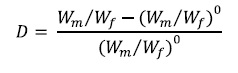
Where is the observed relationship between the male and female wages; and is the women to men wage ratio in the absence of discrimination. If the firms perform in a non discriminating labor market following the principle of minimizing costs, Oaxaca (1973) expresses that:

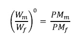
Where PM_m and PMj are the marginal productivity of men and women, respectively; in other words, accepting the neoclassical assumption that an individual's wage is equal to her marginal productivity.

In this sense, Oaxaca (1973) exposes that if there were no discrimination, the wage structure which affects women also could be applied to men, or vice versa.These cases indicate that women, in the absence of discrimination, on average would receive the same salary that men, however discrimination takes the form of women that receive less income than what a nondiscriminatory labor market could give them.

In the particular case of the US economy - as Blinder (1973) mentioned - was very well known that whites earned wages higher than blacks and men earned wages substantially higher than women. Therefore, the assumption that earned wages were equal to the marginal productivity could not hold.

b. Methodology

Blinder (1973) proposes that in order to calculate decomposition it makes sense to estimate first.

The following equations of income for men and women:

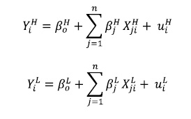
where the H superscript indicates the high salary group [always white men in the study of Blinder 1973] and superscript L indicates the set of low wages group (as alternative, black men and white women). Y_i is the level or natural logarithm of profit, income or wages rate and X1i,... ,XMi are the n observable characteristics used to explain Y

A simple way to calculate the gender wage gap and its causes is to subtract the low-wage group income equation from the high-wage group income equation, assuming that the difference between the

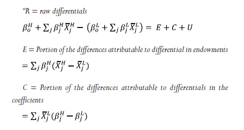
intercepts of the equation corresponds to discrimination²; however, Blinder (1973) proposes that the unexplained portion of the difference comes from both: the differences in coefficients, as the differences in average characteristics of the minority group. Blinder (1973) modeled its proposal as follows:

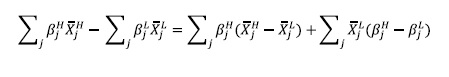
Where the first term represents part of the wage gap that can be explained by differences in the observed characteristics of individuals - endowments possessed - and the second term³ reflects the unexplained portion of the gap, and therefore is interpreted as the effects of discrimination.

In summary, the measures exposed by Blinder (1973) are:

During estimation it must be taken into account that it is critical to use labor incomes of individuals as the dependent variable; this is due to the fact that, in general, surveys include incomes other that labor incomes. On the other hand, selected independent variables depend on the microeconomic wage determination model chosen. Bearing in mind, of course, that correlation does not imply causality, and if the interest is to find the causes of the wage gap you must specify a quite accurate model. (Blinder: 1973)

c. First applications

i. Blinder (1973):

Blinder (1973) in his article, Wage discrimination:reducedform and structural estimates uses wage regressions of white men, black men and white women to analyze the wage differential between black and white men and the wage differential between white men and women.

Blinder (1973) indicates that a part of each wage differential is due to differences in "objective" characteristics such as education and experience, while another part of the differential is not explained by these characteristics. It is all about answering questions about how much of the wage gap between whites and blacks, is attributable to higher education among whites; or how much of the wage differentials between men and women is due to the fact that men may have an easier access to better paid jobs.

To answer these questions Blinder (1973) estimated two equations of income.

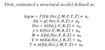
Where w is the wage per hour; Ed is a vector of six educational dummy variables; Occ is a set of eight dummies for occupation; J is a dummy for vocational training; M is 1 for the members of trade unions and 0 otherwise, V is 1 for veterans and 0 otherwise;T is a set of six dichotomous variables for staying in the current work; B is a set of 13 variables of family history; Z is a set of other exogenous variables, and f, g, h, k, l, m and n are linear functions. In this model, w, Ed, OCC, J, M, V y T are taken as endogenous, while B y Z are exogenous. The elements of Z that come into the equation of wages with nonzero coefficients are health, age, residence and the local labor market conditions. Structural estimates -that have a bias unless the error terms are not correlated - were obtained by ordinary least squares⁵.

Additionally, Blinder (1973) estimates the reduced form⁶ of incomes equation using the least squares method, the reduced equation includes B and Z variables that are omitted -explicitly- in the structural equation. Overall, the estimation of the reduced form takes into account individuals' conditions of birth to show the conditional expectation of wages earned by them. For its part, the structural estimates reflect the conditional expectation of income earned by the individual taking into account the current socio-economic status.

By analyzing the income gap between white men and black men, Blinder finds that comparing structural calculations an overall wage advantage of 50.5% of whites over blacks was observed; another finding revealed that 30.7% of the difference (around 60% of the total) is attributable to blacks' lower endowments. Similarly, Blinder (1973) analyzes wage differentials between white men and women and finds that most family history variables used to estimate the structural equation operate in favor of women reflecting its influence through the coefficients.

The coefficients estimated by Blinder showed that white women earn more if they have educated parents and if they were raised in a city in the South, and then in fact they benefited also (while males did not) of having poor parents and being raised on farms. Furthermore, apart from the age, the main advantage white men had was less responsive to local labor market conditions.

According to Blinder, in regressions direct labor market discrimination accounts for around two-thirds of the wage differential and about one third of the difference of the discrimination is due to other endogenous variables, such as labor situation and labor tenure. In other words, it does not attribute any part of the labor differential to differences in labor characteristics.

Having said that, it goes that one of the main conclusions of the work of Blinder (1973) is that, while the differential in salary between whites and blacks and between white women and men was very similar in size, decomposition shows the qualitative nature of the differences by race and sex differed drastically.

ii. Oaxaca (1973):

The income equation estimated by O axaca (1973) for each group (by race and sex) has a "semi-logarithmic functional form as follows:

Where:

Due to the lack of data on the actual number of years of work experience for individuals, Oaxaca defined a proxy for the real work experience that incorporates the model of investment in human capital training. The proxy of experience proposed by Oaxaca is as follows:

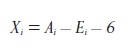
Where X_i is potential experience A_i is the i-th individual's age and E_t the number of years of study approved by the i-th individual. Potential experience and actual experience will match only if individuals obtained their employments immediately after completing their studies; this definition implies that individuals do not experience unemployment, or that individuals didn't work while they studied. For women, the calculation of potential experience has a limitation associated with the time spent on household and child bearing activities. Therefore the potential experience is a reasonable approximation to the real experience of men but exaggerates the actual years of work for women. (Oaxaca: 1973).

In general, it is expected that problems associated with the definition of potential experience don't have a major impact on the estimation of discrimination; however, in an attempt to handle the problem of the missing experience, Oaxaca (1973) included the number of children born to each woman in the analysis. This solution has a problem associated with the correlation between the variables: number of children and potential experience, however, its introduction as a control mechanism was considered necessary.

Other explanatory variables used by O axaca (1973) are defined as follows:

Education: years of schooling completed (linear and quadratic terms);

Class of Worker: dummy variables for union membership (privately employed wage and salary worker), government employed, and self-employed with nonunion private wage and salary workers as the reference group;

Industry: dummy variables for U.S. Census two digit industries with retail trade as the reference group; Occupation: dummy variables for U.S. Census two digit occupations with sales workers as the reference group; Health Problems: dummy variable = 1 if the individual reports health problems that affect the kind or amount of work he or she can perform, and '0' otherwise; Part-Time: dummy variable = 1 if the individual works less than thirty-five hours a week, and '0' otherwise; Migration: a) dummy variable I if the individual has maintained a residence more than fifty miles from his or her current address since the age of seventeen, and '0' otherwise, b)YRSM: number of years since the individual last migrated (linear and quadratic terms); Marital Status: dummy variables for spouse present, spouse absent, widowed, and divorced (or separated) with never married individuals as the reference group; Size of Urban Area: dummy variables for residence in Standard Metropolitan Statistical Areas less than 250,000 (SMSA<250), greater than or equal to 250,000 but less than 500,000 (SMSA 250-500), greater than or equal to 500,000 but less than 750,000 (SMSA 500-750), and greater than or equal to 750,000 (SMSA 750+) with urban, non-SMSA's as the reference group; and Region: dummy variables for U.S. Census regions North East, North Central, andWest with South as the reference group⁸.

The magnitude of the estimated effects of discrimination will depend on the choice of control variables for the wage regressions performed by the researcher; therefore, this election reveals researcher's attitude towards what constitutes discrimination in the labor market (Oaxaca: 1973).

The data used by Oaxaca (1973) came from the Survey of Economic Opportunity of 1967. The used sub-sample was formed by the intersection of: individuals who received a salary per hour in the week previous to the survey; adults aged 16 or older, those living in urban areas, and those who reported their race as white or black.

The results show a chronic gap between working men and women's full time income:

• Calculations based on the wage regressions showed 58.4% discrimination among white men and women and 55.6% among black men and women.

• Furthermore, the effects of discrimination calculated from the regression of wages, personal⁹ characteristics reflected about 77.7% of discrimination for whites and 93.6% for blacks.

d. Critiques:

The econometric regression analysis technique proposed by Blinder and Oaxaca to deduce the causes of the gender wage gap has been subject to considerable criticism that revolves around the model specification and the choice of the independent variables (Riach and Rich: 2002). Below is an outline of these criticisms:

i. Rosenzweig and Morgan (1976) said that the use of age and age squared instead of work experience and squared experience in the structural equation developed by Blinder (1973) creates a differential bias in estimated returns to education for men and is therefore likely that the Blinder results reflect an exaggeration of the size of the component of education that explains the difference in income between men and women attributable to discrimination.

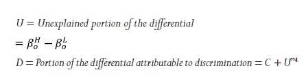
ii. Jones (1983) showed that Blinder's (1973) decomposition method to separate the contribution of the constant term discrimination was defective in the presence of a set of fictional variables, since the magnitude of the estimated constant term depends on the reference out-of-sample group (Oaxaca and Ransom: 1999). In general, Jones (1983) argues that elements U and C of the decomposition proposed by Blinder (1973) are for the most part arbitrary and not interpretable.

What the above discussion shows is that the decomposition of the Blinder's residual term - discrimination - cannot be determined in a unique manner since the value of the difference in intercepts depends on the decisions of measurement. Any specific decomposition using Blinder's algebra will lead to a series of estimates, but the U and C¹⁰ values will always be arbitrary if they depend on the arbitrary decisions of how to set the variables involved in the process of discrimination or, in any social process¹¹.

In response to this criticism, Oaxaca and Ransom (1999) showed that the fundamental problems of identification lay behind the efforts of researchers to estimate separately the contributions that a set of variables have on the component of discrimination. As for the dummy variable, the problem arises from the arbitrary nature of the reference groups that the researcher chooses; fortunately general decomposition and the individual estimates of the effects of endowments are invariant to the choice of reference out-of-sample groups.

However, the problem goes beyond identifying the intercept component. In general, conventional decomposition methodologies cannot identify the single contribution from a dummy variable to the decomposition of wages, because it is only possible to estimate the relative effects of a dummy variable. (O axaca and ransom: 1999) Finally, Oaxaca and Ransom (1999) claim that almost all wage regression models contain categorical variables, so it is unlikely that a detailed application of decompositions can escape the above identification problem.

iii. Other criticism that can be made to the Oaxaca -Blinder approach is that it only measures the discrimination in the labor market. If there are differences in access to endowments that are rewarded in the labor market, -for example; if women have worse access to higher education than men, or even if, ceteris paribus, men are more likely to work than women - then the Oaxaca - Blinder standard approach tends to underestimate the discrimination degree (Madden: 1999).

iv. Furthermore, Atal, Nopo andWinder (2009) although the decomposition Blinder - Oaxaca is the approach most applied in research about wage differentials, it has three noteworthy flaws: First, the decomposition only gives information about the average wage gap omitting the different distribution of this gap among individuals of a same group. Secondly, authors mention that it has been observed that the relationship between characteristics and wages is not necessarily linear, and found that recent data violate fundamental implications of the Mincer model, which is the key input of the decompositions. Finally, the decomposition doesn't restrict the analysis to comparable individuals, which can lead to an upward bias of the component associated with discrimination.

v. From an empirical perspective, the most serious problem that this methodology has is that since estimates of the coefficients capture biases generated from information problems, errors in the variables and selectivity processes, the interpretation of this residual as a means of discrimination is debatable. However, it is worth mentioning that no empirical work is without problems and methodological questions. (Tenjo, Rivero and Bernat: 2002)

e. Methodological improvements

Estimates of wages equations often contain a sample selection bias; this bias arises when non-observed factors that influence the likelihood of participation are correlated with non-observed ones affecting wage. Under such circumstances, the assumptions to ensure the consistency of the estimated coefficients of wage equations are not met, and since the calculation of the percentage of discrimination is based on such estimates, it causes these results to produce wrong conclusions about the degree of wage discrimination against women. (Hernandez and Mendez: 2005)

i. Selection Bias (Heckman:1979)¹²

Heckman (1979) discusses the bias resulting from the use of non-randomly selected samples to estimate the relationships between variables. The author mentions, in contrast to the usual analysis of "omitted variables" in Econometrics, that in the analysis of sample selection bias is sometimes possible to estimate the variables that give rise to specification errors. The estimated values of the omitted variables can be used as regressors allowing estimate behavioral functions which are the interest object of the investigation.

In his article, Heckman (1979) showed sample selection bias as a specification error and presents a simple method of consistent estimation that eliminates the specification error in the case of censored sampling. Heckman argues that sample selection bias may arise in practice for two reasons: first, there may be self-selection of individuals or units of research objects into the data; Secondly, the decisions of sample selection made by researchers or data processors operate almost in the same way of self-selection.

To simplify the exhibition of the characterization of selection bias, Heckman (1979) considers the following two equation model:

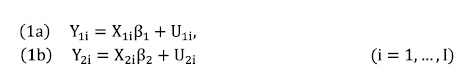
where is a vector of 1 x Kj exogenous regressors, ( is a vector of Kj x 1 parameters and

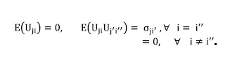
The final assumption is a consequence of the random sampling scheme. Joint density of is (). The regressors matrix is of full rank so if all data were available, each equation parameters could be estimated by OLS.

Heckman proposes the case of estimating equation (1a) but where data does not appear in Y₁ for certain observations, in this case, the critical question is ^why is data missing? The only cost of having an incomplete sample is a loss of efficiency. To estimate the equation it should be aware that:

The population regression function equation (1a) can be written as:

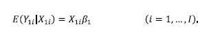
The regression function for the subsample of the available data is:

(i - 1,I)where the convention that the first observations /₁ < 1 have available data for Y_1i has been adopted.

If conditional expectation of U₁ is cero, the regression function of the selected subsample is the same as the population regression function. An OLS estimator may be used to estimate for the selected subsample.

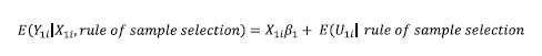
In the general case

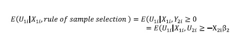
In the case of interdependency between U_1i and U_2i, where data form Y_1i are randomly missing, the conditional mean of U_1i is cero. In the general case, where the mean of U_1i is different from cero the subsample regression function is:

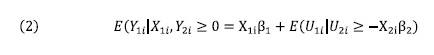
The selected simple regression function depends on X_1i and X_2i. The fitted parameters estimators of equation (1a) in the selected sample omit the final part of equation (2) as a regressor, so that bias resulting from the use of non-randomly selected sample is considered as arising from the common problem of omitted variables.

In the words of Maradona and Calderon (2000) selection bias comes in large part from not observing women that have a higher reservation salary or that have lower opportunity costs of staying at home, or whose characteristics make it more difficult to obtain employment.

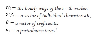
To better understand the effects of selection bias on the estimation of wage differentials, it is assumed that the participation in the labor market depends on the individual's reservation wages. For this reason, if the wage offered by the market is less than reservation wage of the person, it is expected that person decides not to be part of the labor force, while if market wage is greater the individual enter to it. Maradona and Calderon (2000) argue that reservation wage (W_t) depends on individuals' personal characteristics and human capital stock, while the market wage (W_M) depends on human capital only; also, the authors suppose that this dependence is linear and is expressed as:

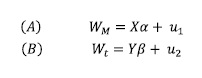
Where X is a vector of characteristics of human capital and Y to a vector of personal characteristics and human capital, and are parameters and, u₁ and u₂ are random errors with zero mean and constant variance.

In words of Maradona and Carlderon (2000), the difference between market and reservation wages represents the propensity of people to participate in the labor market, and is measured by a continuous variable called I and defined as follows:

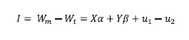
According to this, a woman will decide to join the labor market if this variable takes positive sign. If this is the case, the expected value of the market wage for women will not depend only on the characteristics of human capital (X) but also on the personal features included in the vector Y, which are included in the conditional expectation of the error term. (Maradona and Calderon: 2000).

Maradona y Calderon (2000) exposed that the error term has conditional expectation with zero mean, however, non conditional expectation¹³, which is used when we use OLS, has a non-zero mean and correlates with the independent variables; these are the reasons why the OLS estimates will be biased. (Maradona and Calderon: 2000).

It can be shown that the error term expectation conditional on the participation decision is feasible to breakdown in two terms:

The first corresponds to the ratio of the density function and the cumulative density assessed on the value for each individual function. This term is known as the inverse of the Mill's ratio and is the excluded variable in the analysis of the market wage equation uncorrected for selection bias. The second term is the coefficient of the theoretical regression equations (A) and (B) errors. Thus, the market wage equation corrected for the presence of selection bias in empirical terms is stated as follows:

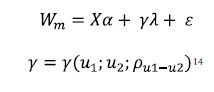
The lambda variable corresponds to the inverse Mill's ratio in particular:

Where Z is a vector of characteristics that determine the probability of labor participation, is a vector of estimated parameter in a probit specification, so that (.) an (.) are the distribution and density functions of a standard normal respectively¹⁵.

The parameter that accompanies lambda is related to the standard deviations and covariance errors in both wage equations. The exclusion of the lambda variable causes a bias in the estimates of the vector. Therefore, estimates are biased unless you enter a value for the variable that corresponds to the probability of being included (or excluded) of the sample of people with income (Maradona and Calderon: 2000).

To resolve this issue, Heckman (1979) develops a method known as two-step estimation method consisting of first estimating a participation equation where a person's decision to participate or not in the workforce depends on a set of personal characteristics, income and human capital variables.This equation is specified ad hoc (Maradona and Calderon: 2000).

In summary, the first stage in the Heckman method consists of a labor participation probit estimation that allows the construction of the variable A that is later included as an additional regressor in the second stage where a wage equation is estimated (Hernandez and Mendez: 2005).

The second stage is the estimate of wages as a function of human capital and the likelihood to participate in the labor market variables - lambda -. The latter is a model for the determination of income a la Mincer, corrected by the presence of selection bias. (Maradona and Calderon: 2000).

ii. The inclusion of correction terms into wage decomposition

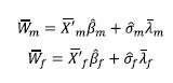
Sample selection bias correction in the estimates of wage equations through the two-step estimation proposed by Heckman (1979) assumes the estimation of the following expressions:

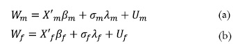
Subscript m refers to the male subsample and f to the female. The variable wage W is a function of the hourly wage, usually the neperian logarithm of the variable; x is a vector of occupational and personal characteristics of the individual with the same components for men and women, ft is the vector of parameters to estimate, A is the correction term (inverse Mill's ratio), (J is the covariance of unobserved factors affecting labor participation and those affecting wage and u is a random perturbation term where E(u)=0. Because the wage discrimination studies use these estimates, selection bias extends to this subject. The OLS estimate which is the second stage allows us to express the known relationship between included variables sample means and parameter estimates. (Hernandez and Mendez: 2005)

The methodology developed in 1973 by O axaca and Blinder allows to break down the wage gap between men and women in two parts of which one is the differential caused by differences in the observed characteristics of individuals; and the other part corresponding to the differential between the wages which is not explained by the characteristics of individuals and therefore associated with discrimination. However, to include the terms of correction, some authors break the salary average difference in three summands, thus:

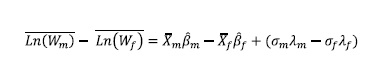
where the bars above variables indicate the estimation of the coefficients at average values of these. Then, adding and subtracting the term gives the following expression:

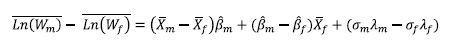
The term corresponds to the part of the wage gap that can be explained by differences in the observed characteristics of individuals. On the other hand, the term reflects the unexplained part of the gap, which is due to differences in the coefficients of X₁ this term is regarded as the effects of discrimination. The term is due to selection bias and is generated by the differences between the incorporation pattern into the labor market men and women have.

Selection bias correction has not been free of criticism. As in Lewis (1986) in most cases there is not a theoretical model to explain the specific selection process, and to specify the variables to explain it. In the absence of this theory, what is usually done is to include ad hoc variables which are thought to be related to that process. This procedure can end up by introducing more problems than it solves in the equations of income. In most cases it is not known if the procedure is capturing the nature of the decisions of individuals, or rather the non-linear effect of variables included in the selection equation. (Tenjo, Rivero and Bernat: 2002)

If the only reason for not reporting income is the fact that people are not involved, you might think of applying the Heckman correction to an equation of a labor participation, whose theoretical support is pretty solid. However, in practice, non report of income may be due to other things (other than non-participation) such as open-wide unemployment or employment in occupations of family assistant without a defined remuneration. This generates additional complications which are not clearly discernible. (Tenjo, Rivero and Bernat: 2002)

f. Applications

i. Gender wage gap

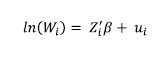
At the international level, several authors have examined the wage differential between men and women and its causes through wage decomposition a la Blinder-O axaca; finding revealing results of the existence of discrimination in most cases. Basically all of these authors estimated mincerian income equations as follows:

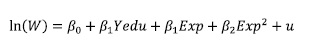
where W is the hourly wage, Yedu represents years of education, Exp years of experience and u is a random error with the usual characteristics (normal distribution, expected value of cero, constant variance, independence of observations and orthogonality to regressors). The majority of cases, in the absence of a measure of actual experience, a measure of potential experience is used.

Expected coefficients derived from these estimates signs are consistent with the hypothesis of the theory of human capital; i.e. an increase in income as years of education increase (positive sign for the variable yedu) and experience (positive sign for the variable exp), but that this effect is non linear, i.e. that the income does not always increase proportionally, but for high levels of experience, the contribution to the increase in income, although positive, diminishes (Bernat: 2005).The use of Heckman's two-step method of estimation is very common to correct selection bias.

We now summarize the findings of research where the gender wage gap was estimated, highlighting where necessary, papers were methodological changes introduced:

• Paz (1998) estimated income gender gap for Buenos Aires and the Argentine Northwest in May 1997. Used data come from the Encuesta Permanente de Hogares (EPH), the studied population comprises all individuals between 15 and 64 years of age (Working Age Population). For the estimation of the regression she always used a weighted sample.

She used two kinds of dependent variables: a) the logarithm of the monthly income (Y); b) the logarithm of the monthly income evaluated at full time (YFULL). In the first case, the matrix of independent variables (X) included as an additional regressor the logarithm of weekly hours worked (LNHOR).

To obtain the variableYFULL she first estimated the following regression for both sexes separately:

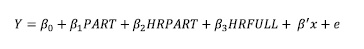
Where PART is a dummy variable to the part-time; HRPART and HRFULL are terms of interaction between the weekly hours of part-time and total, respectively. This adjustment is extremely important given the strong prevalence of female workers in part-time labor. Using the estimated coefficients for PART, HRPART and HRFULL, YFULL was constructed according to equation:

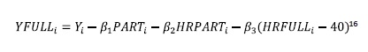
In the words of the author, the fundamental property of this variable is that it "punishes" income of those working more than 40 hours per week and "rewards" income of part-time workers, i.e., homogenizes the equivalent to 40 hours per week for the market income.

The obtained results showed that the differences in the gap between Gran Buenos Aires and the Argentine Northwest were small and it is likely that they respond more to the rounding of numbers rather than economically relevant issues. Observed gap is located in not less than 0.70 or more than 0.85, depending on the specification of empirical models used to estimate them. The portion of the gap that is not explained by the endowments of human capital and occupational position does not differ between the two labor markets and is situated in the order of 90% approximately (Paz: 1998).

• In the case of Latin America, Tenjo, Rivero and Bernat (2002) analyze the evolution of wage differences by sex in Argentina, Brazil, Costa Rica, Colombia, Honduras and Uruguay in the estimation of the mincerian equations for men and women, employeed and unemployed, for each of the six countries in study, using wage differentials Oaxaca decomposition.

The authors estimated Mincer equations for men and women, with and without selection correction, for employed and unemployed, for each of the six countries in the study.The dependent variable used was the hourly income; to correct for selection, an estimation of Heckman's two-step method was used.

The authors come to the conclusion that there are differentials in monthly salaries between men and women, that these have declined significantly in favor of female workers, and also that the immediate reason why women have lower monthly wages than men is because they work fewer hours.

Similarly, Tenjo, Rivero and Bernat (2002) observed a significant level of job segregation by branch of economic activity and occupations. However they make clear that this segregation is not reflected in lower wages for women. Thus, hourly wage differentials between men and women appear to be associated with labor remuneration patterns within sectors and occupation.

• Di Paola and Berges (2000), calculated the gender wage gap estimating income Mincerian functions for both sexes and applying the technique of Blinder and Oaxaca.

The dependent variable, the logarithm of the monthly hours, was calculated from the hours per week declared in the Survey¹⁷ by the worker, divided by 7 and multiplied by 30. They expected that signs and approximate values of the coefficients of the income function matched the hypothesis of human capital. The authors also stated that the coefficient of the natural logarithm of monthly hours worked should be positive and it would be interpreted as an elasticity, indicating in what proportion varies the income to a percentage change in hours worked (Di Paola and Berges). They corrected the problem of selection bias by estimating labor participation equation as mentioned above.

The model suggested by Dipaola and Berges (2000) for selection bias correction was as follows:

Where, Parti is female labor market participation (Dichoto-mous variable = 1 if the woman receives labor income and 0 = otherwise), is woman's age, is age squared, S_i are years of schooling, Est1₁ indicates 1st stratum, eEst2₁ indicate 2^nd stratum,Yjefe₁ is head of household's income, N_i is the number of house members, n_i is a residual term, subscript i indicates woman i = 1,........,548.

The results show that: if results were not corrected and if women were paid as men, the total difference of the logarithm of income would be 0.471. After performing the difference decomposition, 28% is explained by the allocation of human capital and the remaining 72% by the market structure. Estimates for this income selection bias-corrected equation yielded different results. The total difference of the logarithm of the income is lower, 0.196 and reverses the relative importance of the components that explain (human capital 78% and 22% market structure) (Di Paola y Berges, 2000).

• Johanson, Katz and Nyman (2005) discuss the evolution of wage differentials and the factors that may be related, year by year through the analysis of cross section data of the Department of statistics of Sweden (HEK) for the years 1981 and 1983-98; therefore decompose the wage differential gender according to the standard method of Oaxaca (1973).

The dependent variable on estimates is (the logarithm of) imputed hourly wage. Variables used in the wage equations are age squared, fictional variables for: the level of training, requirements to be a blue-collar or white-collar worker, industry, region, the central government, the private sector, or local government employees and to work in men-dominated or women-dominated occupations (Johanson, Katz and Nyman: 2005). Authors view age as a measure of the experience of life in general, that can affect the wages.

The results showed that the difference between the geometric average wages per hour of men and women ranked between 13 and 14 per cent of the average wage of men during 1983-1987. From 1988 it was around 14-16%, except for a gap of 17 per cent in 1990 (Johanson, Katz and Nyman: 2005).

• Bernat (2005) analyzed the wage differential per hour between men and women in seven major metropolitan areas of Colombia in the period 2000-2004; attempted to explain the change in the differential in these years, distinguishing two components: on one side, the contribution that can generate human capital differences, and on the other, a discriminatory component, understood as anything that is not explained by differences in the first contribution (Bernat: 2005).

Bernat (2005) estimated wage decomposition of O axaca-Blinder correcting for selection bias, therefore, first estimates the participation equation, using variables such as marital status, head of the household, the unemployment rate of the family and the number of children, characteristics which clearly affect the participation of an individual in the labor market. The income for the rest of the family is included as an approximation of the individual's reservation wage. The higher this income, the higher it is expected that the individual has more time to analyze employment opportunities in the labor market, the crossover effect (cc) that it includes investigates whether being a married head of the household or unmarried household head affects the decision of labor market participation. (Bernat: 2005).

Among cities, the hourly wage differentials (only salaried workers) were lower in Manizales, Bogota and Medellin. For the seven cities considered total, discrimination was at 20% for salaried and 21% in average for non-salaried, in the period under review, although with different aggregate trends and between cities for the two groups (Bernat: 2005).

ii. Other applications

This section summarizes the work of several researchers who estimated wage gaps by ethnicity, nationality, among others:

• Johnson (1978) estimated wage discrimination by industry using a broad sampling of data on the individual characteristics of the worker, the industrial employment and wages. This work aims to investigate how competitive features of an industry influence its tendency to engage in wage discrimination. Johnson (1978) measured the wage discrimination due to the residual difference between the salaries of blacks and whites that is not due to their personal characteristics.

The estimated equation is as follows:

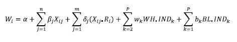
Where,W_i is the salary for the i-th individual, X_ij are personal characteristics, are market determined parameters, X_ij ^. R_i are interaction terms with race and a group of m < n characteristics, that represent the interaction of dummy employment variables for whites and blacks in the industry k, (k = 1... P).

Racial discrimination by industry estimates are calculated by , meaning; the wage gap between whites and blacks in the same industry, after discounting the differences in the individual characteristics¹⁸

According to the results found by Johnson, employers classified as costs minimicers discriminate more in wages that employers who can operate more independently of the competitive market discipline. The regulated companies seem to discriminate less than other for-profit employers.

• Stewart (1983) attempts to provide empirical evidence about the differences in occupational positions between black and white immigrants born in the United Kingdom that have the same personal characteristics and only differ by their country of birth. This research, only examines the discrimination in the labor market and therefore the results may be less than total discrimination, due to the origin of the individuals. Also, the author indicates that differences attributed to discrimination are the result of a combination of race discrimination and discrimination on the basis of the country of birth.

According to the author, estimated results revealed that between 75 and 100% of the differential average income was caused by differences in occupational level, indicating the problem refers to the policy of entry to work instead of different payments within a same occupation level. In spite of changing economic conditions, no evidence of movements on the average wage differential in the period 1970-1975 was found. Finally, noted that during this period black immigrants have progressed considerably less, professionally, than whites born in the United Kingdom. (Stewart: 1983)

• Reimers (1983) attempts to measure the degree of wage discrimination against Hispanics and Blacks in the United States. The author uses microdata from the Survey of Income and Education from 1976 to estimate separate wage functions, selection bias corrected for each ethnic group -Mexican, Puerto Rican, Cuban, Central American and South American, other Hispanic, non-Hispanic and white non-Hispanic blacks. Samples consist of wages for employed male civilians, 14 or older, who were not self-employed or full-time students.

According to the author, the differences in average income can be decomposed as this:

Where I is the identity matrix and D is a weighting diagonal matrix.

Reimers found that for men of Puerto Rico, discrimination may be responsible for 18% of the wage differential, on its part, for "other Hispanics", discrimination can cause up to 12% of the wage gap. For Mexicans, however, accounts of discrimination only amount to 6%, the rest of the 34% wage gap is due to differences in characteristics such as education (Reimers: 1983).

2. CONCLUSIONS

In this article we make an effort to illustrate a technique for the analysis of wage discrimination. We first expose the independent works of Blinder (1973) and Oaxaca (1973), followed by criticism and methodological improvements it has experienced over time. We also summarize empirical implementations of the technique for the analysis of gender and racial discrimination.

Estimates of wage differentials between groups of individuals - minority-majority - has been well studied; understanding what explains this gap led Blinder (1973) and Oaxaca (1973) to devise -independently - a way to break down the wage gap into two summands: one explained by the characteristics of individuals and another explained, allegedly by discrimination.

This methodology has been widely used, in spite of its limitations and disadvantages, especially to calculate the wage differential between men and women and to demonstrate the existence of discrimination as a key cause of those differences. A methodological improvement by many researchers is to include a third summand representing the existence of selection bias in the sample; this term is entered using the estimate proposed by Heckman's two-step method in 1979.

Subsequently, several authors have developed a few extensions of the original method proposed by O axaca and Blinder; however, the analysis of these methodologies was not addressed in this article due to its lengh. Therefore, an analysis of the methodologies that extend the original conception of wage decomposition of O axaca - Blinder is proposed as a topic of interest and will be carried out in a subsequent paper, where we will review techniques that focus not only on average differences but that also decompose, indexes and distribution functions.

¹ Blinder, Alan S (1973), "Wage Discrimination Reduced Form and Structural Estimates", Journal of Human Resources. Vol 8, N.° 4. Pág 438.

²As follows: 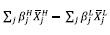and the quantity that is captured by the intercepts this last expression used be attributed to discrimination.

³ In words of Blinder (1973) the second part is the difference between how the high salaries equation values the features of low wages group and how the equation of low wages really values it

⁴ Ibid. Pag 439.

⁵ Ibid, Pag 441.

⁶The reduced equation is log w = F(B,Z) + v₁

⁷ Oaxaca, Ronald L (1973), "Male-Female Wage Differentials in Urban Labor Markets", International Economic Review, 9. Pag 695.

⁸ Ibid, pag 698.

⁹ It refers to a set of equations that not control by occupation, industry and the class of workers class.

¹⁰ U = Unexplained portion of the differential Portion of the differences attributable to differentials in the coefficients

¹¹ Jones, F. L (1983), "On Decomposing the Wage Gap: A Critical Comment on Blinder's Method," Journal of Human Resources 18. Pag 130.

¹²We reproduce Heckman's original exposition in order to facilitate reader's understanding.

¹³

¹⁴ Maradona, Perlbach y Calderon, Monica, "Estimacion del sesgo de selection para el mercado laboral de Mendoza", Facultad de Ciencias Econo-micas, Universidad Nacional del Cuyo, p. 7.

¹⁵ Hernandez, Pedro y Mendez, Ildefonso (2005) "La correction del ses-go de selection en los analisis de corte transversal de discrimination salarial por sexo: estudio comparativo en los paises de la Union Europea" , Estadis-tica Espanola, Vol. 47, Num. 158, p. 183.

¹⁶ Paz, Jorge (1998), "Brecha de ingresos entre generos. (Comparacion entre el Gran Buenos Aires y el Noroeste Argentino)". 19 p.

¹⁷The Information used came from the wave of May 1997, of the Permanent Survey of Homes made by the INDEC for the area of Mar de la Plata.

¹⁸ Johnson, William (1978), "Racial Wage Discrimination and Industrial Structure" The Bell Journal of Economics, Vol. 9, No. 1. Pag 72.

REFERENCES

Atal, J., Ñopo, H. & Winder, N. (2009). New Century, Old Disparities: Gender and Ethnic Wage Gaps in Latin America. IDB Working Papers, 109, 76.         [ Links ]

Bernat, L. (2005). Análisis de género de las diferencias salariales en las siete principales áreas metropolitanas colombianas: ¿Evidencias de discriminación? Cuadernos PNUD – DANE.         [ Links ]

Blinder, A.S. (1973). Wage Discrimination Reduced Form and Structural Estimates. Journal of Human Resources, 8, (4), 436-455.         [ Links ]

Di Paola, R. & Berges, M. Sesgo de selección y estimación de la brecha por género para Mar del Plata. Centro de Investigaciones Económicas - Universidad Nacional de Mar del Plata.         [ Links ]

Heckman, J. (1979). Sample Selection Bias as a Specification Error. Econométrica, 47, 153-161.         [ Links ]

Hernández, P. & Méndez, I. (2005). La corrección del sesgo de selección en los análisis de corte transversal de discriminación salarial por sexo: estudio comparativo en los países de la Unión Europea. Estadística Española, 47, (158), 179-214        [ Links ]

Johansson, M., Katz, K. & Nyman, H. (2005). Wage Differentials and Gender Discrimination: Changes in Sweden 1981-98. Acta Sociológica, 48, (4), 341-364.         [ Links ]

Johnson, W. (1978). Racial Wage Discrimination and Industrial Structure. The Bell Journal of Economics, 9, (1), 70-81.         [ Links ]

Jones, F. L. (1983). On Decomposing the Wage Gap: A Critical Comment on Blinder's Method. Journal of Human Resources, 18, 126-130.         [ Links ]

Madden, D. (1999). Towards a Broader Explanation of Male-Female Wage Differences". Centre for Economic Research. WP99/11, 15.         [ Links ]

Maradona, P. & Calderón, M. Estimación del sesgo de selección para el mercado laboral de Mendoza. Facultad de Ciencias Económicas, Universidad Nacional del Cuyo.         [ Links ]

Oaxaca, R. L. (1973). Male-Female Wage Differentials in Urban Labor Markets. International Economic Review, 9, 693-709.         [ Links ]

Oaxaca, R. L. & Ransom M. R. (1999). Identification in Detailed Wage Decompositions. The Review of Economics and Statistics, 81(1), 154-157        [ Links ]

Riach, P. & Rich, J. (2002). Field experiments of discrimination in the market place. The Economic Journal, 112, F480–F518.         [ Links ]

Reimers, C. (1983). Labor Market Discrimination Against Hispanic and Black Men. The Review of Economics and Statistics, 65, (4), 570-579.         [ Links ]

Rosenzweig, M. & Morgan, J. (1976). Wage Discrimination: A Comment. Journal of Human Resources, 11, 3-7.         [ Links ]

Palacio, J. & Simón, H. (2006). Segregación laboral y diferencias salariales por razón de sexo en España. Estadística Española, 48, (163),493-524.         [ Links ]

Paz, J. (1998). Brecha de ingresos entre géneros. (Comparación entre el Gran Buenos Aires y el noroeste argentino).         [ Links ]

Stewart, M. (1983). Racial Discrimination and Occupational Attainment in Britain. The Economic Journal, 93, (371), 521-541        [ Links ]

Tenjo, J., Ribero R. & Bernat, L. (2002). Evolución de las diferencias salariales por sexo en seis países de América Latina. Colección Documentos de Economía 1, 59.         [ Links ]

Tenjo, J. & Herrera, P. (2009). Los ensayos sobre discriminación: discriminación salarial y discriminación en acceso al empleo por origen étnico y por género, Colección Documentos de Economía 1.         [ Links ]