


 English (pdf)
 Article in xml format
 Article references
 Send this article by e-mail
 Cited by SciELO
  Cited by Google
  Similars in
SciELO
Similars in
SciELO  Similars in Google
 Permalink
1. Introduction
The use of non-invasive and non-destructive optical systems in crop inspection and control, helps producers to improve integral agricultural management practices and control phytosanitary risks, by providing information that allows a correct diagnosis of problems with potential damage to agricultural production. Within these optical systems, hyperspectral sensors have allowed the detection of phytosanitary problems at early stages and the elimination of the incidence of the human factor in its detection. Hyperspectral images (HSI) provided by these sensors, have been used in recent years for the development of: non-invasive and non-destructive fruit inspection methods (dos Santos Netoa et al., 2017; Munera et al., 2017; Pinto et al., 2019); the establishment of spectral vegetation indices to estimate internal damage in harvested fruits (Vélez-Rivera et al., 2014); and the early detection of crop diseases (Zarco-Tejada et al., 2018; Navrozidis et al., 2018).
However, as in any sensors and measuring instruments, the captured data are subject to anomalies that can alter the information contained in them and, therefore, skew the results obtained. Techniques such as MNF or PCA, have been applied in numerous studies, which is why these techniques are presented as necessary steps in all hyperspectral analysis. For example, Bjorgan & Randeberg (2015), developed an MNF technique applied to pushbroom hyperspectral images for spectral denoising during real-time image acquisition. The authors of this work affirm that the results obtained with this technique, are comparable to those obtained after acquiring the image in its entirety. Moreover, Liao et al. (2013), proposed a two-phase model that combines a kernel PCA (KPCA) and a model for eliminating total noise variation that evidenced remarkable characteristics and promising results as far as denoising is concerned.
In recent years, techniques based on deep learning networks (Yuan et al., 2019), and bilinear factorization (Chen et al., 2020), have been applied to HSI for noise detection. Yuan et al. (2019), presented a technique based on a deep convolutional neural network that combines space and spectrum through an end-to-end mapping between clean and noisy HSIs. The results reported with this technique are outstanding when compared with traditional methods, although its validation was carried out partly with simulated data. Fan et al. (2019), proposed a method based on bilinear low-range matrix factorization (BLRMF), where the binuclear quasi-standard is used to restrict low-range characteristics, which are supposed to contain the noisy signals in HSI. Based on the area covered by Fan et al. (2019), Chen et al. (2020) proposed a technique based on bilinear factorization regularized by total variation and conducted numerical experiments with 5 different types of mixed noise scenarios and 1 with real data.
The state of the art reports a wide variety of techniques and approaches to solving the problem of noise detection and removal in HIS. However, to the best of our knowledge, an approach purely based on the discrete wavelet transform has not been explored in sufficient detail. For this reason and considering the importance of this problem in HSI, this paper presents the study, comparison and implementation of three algorithms (Hard Thresholding, Soft Thresholding and Neigh-Shrink), based on the discrete wavelet transform. These algorithms were tested with a bank of 180 hyperspectral images acquired from mango samples (leaves) that were subjected to phytopathological studies for the detection of anthracnose in mango. As a result, it was found that the techniques exposed present a good performance in terms of spectral denoising. The Neigh-Shrink technique obtained the best performance.
The remainder of this article has the following structure. Section 2 details the materials used as input for the development of this work and the methods of denoising in the HSIs studied. In section 3, the results obtained in each test are presented and discussed in terms of the spatial and spectral components since the images are susceptible to the presence of noise in both components. Finally, section 4 outlines the main conclusions.
2. Methods
2.1 Samples and image capture system
For the development of the study, mango leaves (Mangifera Indica L.) of the Tommy Atkins and Keitt varieties were used from a producing farm located in Anapoima, Colombia (4°35'21.4" N 74°31'07.6" W). From this crop, 45 mature leaves were pre-selected per variety from the middle third of trees with an average life of 4 years. From these groups of leaves, 15 of them were selected per variety, for a total of 30 leaves used in the study.
The vision system used for capturing hyperspectral images corresponds to a Hyspex VNIR-1600 pushbroom sensor (Hyspex by Neo, Norsk Elektro Optikk,Norway), with spectral resolution of 3.629383 nm, 1600 spatial pixels and range of 400-1000 nm, obtaining 160 spectral bands per scan. The images were taken in a controlled environment. The hyperspectral sensor was placed on the leaf at a distance of 30cm, which was illuminated with a halogen light source VNIR of 150W at 45 ° on the plane where the sample to be photographed is located.
Each leaf was placed on a black background, with a calibration panel and a label located at the top of the scene to identify the sample photographed. Figure 1 presents an RGB image extracted from the hyperspectral image showing the disposition of the sample.
Figure 1 Hyperspectral image in RGB of a mango sample with identification label and calibration panel on top.
Each group composed of 5 samples was photographed daily from 24 to 29 November 2019. Therefore, 6 hyperspectral images were obtained per sample for each variety of mango, resulting in a bank of 180 images to be processed (90 per variety). Finally, each image had a dimension of 1600x3800x160 (width, height, spectra) encoded in 2 bytes per pixel.
2.2 Denoising methods
The problem of additive denoising in images (standard, monochromatic, hyperspectral, among others), can be addressed with the assumption that an X image can be decomposed into:
Where S represents the matrix with the image signal and Σ represents the noise in the image. Both matrices kept the same dimension. In the case of a monochromatic image matrix, S and Σ would have dimensions (I1, I2), while in the case of RGB images there would be matrices with dimensions (I1, I2, 3). This behavior can be extrapolated to larger images (as in the case of hyperspectral images), where images would have dimensions (I1, I2, I3), being I1 and I2 the spatial dimensions and I3 the spectral dimension.
However, within dimension I3, which in this study corresponds to the spectral dimension and has a value of 160, there are bands that usually contain a high signal-to-noise ratio (SNR) and others that, on the contrary, have a low SNR and are highly noisy, hence, they are discarded from the dataset to be analyzed. These highly noisy bands are known as junk bands (Heylen et al., 2011), and lead directly to the total loss of the information contained in them, which means a loss of the captured data. With this intrinsic noise problem, there is a risk that the proposed spectral study be biased since it does not have all the data initially captured. Therefore, a method that allows the detection and reduction of noise in images is a necessary step in hyperspectral analysis.
In this context, this paper implements a denoising technique based on the discrete wavelet transform, an approach commonly used in the analysis of signals and computer vision, but scarcely applied to hyperspectral analysis.
Identification of noisy bands
As the spatial and spectral resolution of hyperspectral images (HSI), decreases and the number of bands that such an image can contain increases, the correlation between adjacent bands increases too (Zelinski & Goyal, 2014). This correlation applies not only to the signal itself but also to the noise of the image, which can be highly correlated between adjacent bands (Farzam & Baheshti, 2011). In HSI, this spectral correlation is usually much stronger than the spatial correlation in standard images. The reason is that the same pixel represents the same object along different bands, while an adjacent pixel at the spatial level can represent another object that is not necessarily correlated to the analyzed pixel. For example, Figure 1 shows a leaf where an adjacent pixel in the spatial component can correspond to the background of the scene, while a pixel on the leaf is composed of the different spectral bands that comprise the hyperspectral image.
To measure the spectral correlation between two bands, at the numerical level, the linear correlation coefficient or Pearson's coefficient was defined as:
Where i and j are two different bands of the hyperspectral image. To define the appropriate correlation level in a neighborhood surrounding a band i, the number B of adjacent bands was defined, in which the Pearson coefficient contains the information provided by the B bands adjacent to band i. If the correlation coefficient is less than a threshold t, the band is said to have no correlation with the surrounding bands and will therefore be a highly noisy band (or junk band). For calculating Pearson coefficient, Karami et al. (2014), suggest that the t-value should be 0.9, while the value of B is set in 7.
Discrete wavelet transform in 2D
The discrete wavelet transform outputs are two sets of data: one set gives information about the low frequencies (L), while the second one about the high frequencies (H) of the signal. Generally, the vast majority of the information that describes the signal is immersed in the low frequency L data.
The algorithm of the 2D discrete wavelet transform separates the image into rows and columns. In the first step, the transform is applied to all rows (horizontal transform), thus obtaining 2 initial sets, L and H. Each of these sets is half its original size. Subsequently, the procedure is repeated in the columns of the two images resulting from the previous step. From these images, a set L and H is also obtained, that is, there will be 4 sets: LL, LH, HL, HH. Each of them will be a quarter of the size of the original image. This process is repeated until the desired resolution is obtained. The resulting matrix has the form shown in Figure 2.
Each level of transformation has bands of coefficients with high frequency components in the set H. These coefficients are usually filtered with different techniques, since they usually preserve a greater part of the noise components of the signal (Chen et al., 2005). In this study, three filtering methods of high frequency coefficients (Hard Thresholding, Soft Thresholding and Neigh-Shrink) were analyzed, with the aim to obtain the best reconstruction of the hyperspectral cube without the spectral and spatial noise captured in the collecting phase of hyperspectral images on mango samples.
Method of filtering for high frequency coefficients
There are several methodologies to perform the filtering of high frequency coefficients. However, three main methods are usually used as the basis for denoising: Hard Thresholding, Soft thresholding and Neigh Shrink algorithm.
Hard Thresholding filtering method. The Hard Thresholding method has a working principle similar to that of the binary thresholding function: any value below a certain threshold will be taken as the zero value, while the others will be kept unchanged. Mathematically, the Hard Thresholding operator is defined as:
Where λ is the chosen threshold value and w is the value of the matrix of high frequency coefficients. The function of Hard Thresholding is illustrated in Figure 3(a).
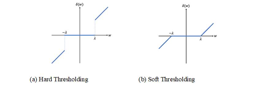
Soft Thresholding filtering method. This method works similarly to Hard Thresholding with the difference that greater values than the threshold are recalculated by subtracting the threshold value. On the other hand, values below the threshold are equal to zero, as proposed by the Hard Thresholding method. Mathematically, the Soft Thresholding operator is defined as:
Where λ is the chosen threshold value, sgn is the sign function, and w is the value of the matrix of high frequency coefficients. Figure 3(b) shows the graphical behavior of the Soft Thresholding function.
Neigh-Shrink filtering method. The Neigh-Shrink method aims to estimate a value of high frequency coefficients without noise, defined as:
Where
Where the + sign indicates that the value of β will only be taken into account if it is positive, and it will be equal to zero if it is negative. The term λ is the value of the threshold,
Selecting the threshold value. The common element of the three methods described above is the threshold value λ. The Universal Threshold has been defined as:
Where
Where w s refers to the values belonging to the sub-band HH, HL or LH to be treated. By defining the thresholding value, it is possible to implement and analyze the denoising methods discussed in this work.
3. Results and discussion
Laboratory hyperspectral images, acquired under controlled conditions, present low noise levels in the captured scene (Figure 1). To magnify the presence of noisy bands and facilitate denoising through the wavelet transform, a gaussian noise addition stage was executed, with levels of σ=10, 20, 30, 40 and 50 and taking into account that the maximum grey scale of the image per spectral band is 255. With the above conditions, the aim is to adequately compare the performance of the techniques presented in section 2.2, and define the best denoising scheme for hyperspectral images.
Each of the methods was tested with different iterations of decomposition (1, 2, 3 and 4 iterations) using the discrete wavelet transform. The selection of these values corresponds to previous tests indicating that more than 4 iterations produced no significant improvement in the denoising of the image. Figure 2 illustrates the decomposition performed by the transform at each iteration.
As a criterion for measuring the quality of the filtering, Peak Signal-to-Noise Ratio (PSNR) was used for denoising in the spatial component. This metric is commonly used in this field since it represents the relationship between the maximum power of the image and the noise that affects it. Regarding the spectral denoising component, SNR was used as a metric, since no signals without noise (or with a low level of noise), are required to quantify it, in contrast to the spatial component.
Finally, the three denoising methods based on the discrete wavelet transform (Hard Thresholding, Soft Thresholding and Neigh-Shrink) were tested in the bank of 180 hyperspectral images. This means that each algorithm processed 28,800 monochromatic images resulting from the decomposition of each hyperspectral image into the 160 spectral bands.
3.1 Denoising in the spatial component
With Hard Thresholding, it was found that when the noise is low, with σ = 10, the best result is obtained with 1 iteration of the transform (Table 1). Although the result is numerically better than in the cases of 2, 3 and 4 iterations, the improvement with respect to the worst case (4 iterations) is barely 2.5% (Table 1).
Table 1 PSNR for different levels of decomposition and noise using Hard Thresholding.
| п | PSNR (dB) 1 iteration | PSNR (dB) 2 iterations | PSNR (dB) 3 iterations | PSNR (dB) 4 iterations |
|---|---|---|---|---|
| 10 | 30.65 | 30.34 | 30.02 | 29.90 |
| 20 | 26.40 | 27.18 | 26.90 | 26.74 |
| 30 | 23.71 | 25.39 | 25.33 | 25.14 |
| 40 | 21.57 | 24.06 | 24.24 | 24.01 |
| 50 | 19.82 | 23.00 | 23.44 | 23.24 |
When the noise level increases with σ ≥ 20, a single iteration with the transform is no longer enough to obtain good results. This trend becomes apparent in Figure 5, where the PSNR values decay as the noise in the image increases. PSNR values are more pronounced when the method performs 1 iteration (blue line); while for 2, 3 and 4 iterations the results are relatively better and quite similar to each other, since they manage to maintain better levels of PSNR.
In the case of the Soft Thresholding method, the results showed similarity to those from Hard Thresholding: 1 iteration yields better results only when the noise level is low, however, when the noise level increases, it is also necessary to increase the number of iterations in order to obtain good results (Table 2). In this case, similar trends are also obtained for 2, 3 and 4 iterations, although the difference between the lines that describe their results (Figure 6) do not converge in the same way as in Figure 5. As an advantage over Hard Thresholding, this behavior allows differentiating the appropriate number of iterations for the transform and the method for different noise levels.
Table 2 PSNR for different levels of decomposition and noise using Soft Thresholding.
| п | PSNR (dB) 1 iteration | PSNR (dB) 2 iterations | PSNR (dB) 3 iterations | PSNR (dB) 4 iterations |
|---|---|---|---|---|
| 10 | 29.87 | 28.52 | 27.64 | 27.29 |
| 20 | 26.37 | 26.21 | 25.23 | 24.71 |
| 30 | 23.71 | 24.84 | 23.96 | 23.33 |
| 40 | 21.57 | 23.81 | 23.23 | 22.49 |
| 50 | 19.82 | 22.92 | 22.65 | 21.89 |
Finally, the trend observed in Figures 5 and 6 with the two previous filters changed with the Neigh-Shrink method. The data obtained for this technique are shown in Table 3 and Figure 7. With 1 iteration, the PSNR decreases rapidly as the noise level increases, which indicates low robustness against external noise. But with 2 and 3 iterations this method proved to have better performance with low noises (σ =10) and a remarkable performance in the presence of noise levels σ ≥ 20, since the PSNR level does not decrease drastically as in the case of 1 iteration. Additionally, with this technique PSNR levels decline with 4 iterations, thus demonstrating that no more than 3 iterations are needed to obtain the best results, in terms of detection and reduction of noise in a hyperspectral image.
Table 3 PSNR for different levels of decomposition and noise using Neigh-Shrink.
| п | PSNR (dB) 1 iteration | PSNR (dB) 2 iterations | PSNR (dB) 3 iterations | PSNR (dB) 4 iterations |
|---|---|---|---|---|
| 10 | 31.96 | 32.84 | 32.43 | 31.24 |
| 20 | 26.88 | 28.73 | 28.94 | 28.13 |
| 30 | 23.82 | 26.47 | 26.98 | 26.73 |
| 40 | 21.60 | 24.88 | 25.79 | 25.67 |
| 50 | 19.83 | 23.58 | 24.82 | 24.83 |
An overview of the results indicates that a greater the number of decompositions (such as those shown in Figure 3), produces better results and higher PSNR values. However, a more detailed analysis of the data contained in Tables 1, 2 and 3 indicates that the best results for each filter were obtained with 2 and 3 iterations. The only case that differs from this behavior is with the Neigh-Shrink filter for σ=50, however, the improvement of the PSNR obtained with 4 iterations represents only 0.3% compared with 3 iterations. Consequently, it is inferred that improvement in the noise filtering quality with the discrete wavelet transform is not directly proportional to the number of iterations. A very high number of iterations could even force the algorithm to perform unnecessary filtering and there would be a significant waste of information, which is relevant in the case of hyperspectral images as it is directly related to the reflectance level of the sensed objects.
Based on the above and on the performance comparison of the filters (Tables 1, 2 and 3), it was observed that the highest PSNR levels were obtained with the Neigh-Shrink method, followed by Hard Thresholding and Soft Thresholding. Moreover, considering that the presence of noise in hyperspectral images acquired under laboratory conditions is low but significant, the configuration of the Neigh-Shrink method with σ=10 showed promising results as it resembles the noise originally contained in this type of images. Finally, the Neigh-Shrink method should be configured to work with 3 iterations for noise treatment in hyperspectral images.
3.2 Denoising in the spectral component
To identify the presence of noise in a spectral signature, it is necessary to take into account the high correlation between adjacent wavelengths (bands). Figure 8 shows the correlation of the 160 bands of an acquired hyperspectral image. It is worth noting that the main diagonal, which is colored in yellow and ideally should be a line, is represented with greater thickness than that of a line, which allows assuming the correlation level that between adjacent bands is greater than 0.95. This value was used as the initial parameter for the identification of noisy bands in the hyperspectral images acquired for this study.
However, after the identification of noisy bands, it was found that this threshold was not able to detect bands that could contain noise. An explanation for this phenomenon, lies in the foregoing fact of the high correlation between bands that hinders the sensor from capturing the reflectance changes between one band and another, even though the sensor is designed to do so. Another possible explanation is the presence of spectral noise that induces distortion of two or more adjacent spectral bands in their real reflectance level. For this reason, it is necessary to find the appropriate level of correlation between bands, to detect which of them may be subjected to a noise that must be eliminated.
Due to the consequences that the presence of noise in the spectrum can cause, the level of correlation between neighboring bands was gradually increased to 0.99. It was found that until this value (0.99) it is possible to detect bands that were classified as noisy. In particular, the wavelengths found were: 417.56, 421.19, 969.22, 980.11, 983.74, 987.37, 991.00, 994.63, which are particularly located at the ends of the spectrum (Figure 9a). This finding is explained by the noise induced by the sensor when capturing the spectral data. According to Hyspex, the manufacturer of this sensor, the efficiency curve in the capture of spectral data is affected at the ends, that correspond to the moments of start and ending of capture of the sensor. Additionally, electrical factors, such as voltage fluctuations affecting both the sensor and the computer equipment or lighting source, can induce alterations (noise) in the recorded data.
Although the ends of any special signature are generally eliminated in spectrum analyses, each spectrum, each band and each datum, counts when exploratory scientific studies are performed, e.g. spectral characterization of diseases in plant material. Therefore, the correction of these alterations (noise) is achieved using the discrete wavelet transform, which allows considering the entire spectrum in each hyperspectral image. Figure 9 shows a comparison of an uncorrected spectral signature (Figure 9a) with respect to the corrections made by the 3 methods studied (Figures 9b, c, d). In the original signature, the ends present alterations (or noise), which correspond to the noisy bands found, whereas the signatures filtered by each of the methods manage to reduce the amplitude of these alterations, thus achieving a better quality in the spectral signatures obtained. Although there are some remaining peaks, they are small compared with those in the original image and may correspond to specific spectral characteristics of the leaf, so aggressive denoising could eliminate these alterations that can be valuable in hyperspectral studies. These findings validate the selection of the number of iterations of the applied transform.
Figure 9 Spectral signature of a pixel in the hyperspectral image of a leaf (a) before and after (b) Hard Thersholding, (c) Soft Thersholding and (d) Neigh-Shrink filters.
At the quantitative level, when the SNR of each band was calculated, the results obtained (Figure 10) were conclusive and validate the above findings. The SNR of the original bands reaches 74.04 at its highest point (Figure 10a) and is located in the middle zone of the spectrum (bands with less noise), while at the ends it decreases considerably, which is plausible since these areas showed greater presence of noise in the spectral signature. Besides, when the three denoising filters are applied, the SNR increases considerably in all cases (Figures 10b, c, d), thus reaching the scale of 1011. With these filtering methods, it is also observed that the intermediate bands have a lower SNR with respect to the ends. This is consistent with the fact that these areas of the spectrum will undergo more corrections by the filters since they have a higher level of noise, which causes them to have a higher SNR after filtering.
Figure 10 SNR of the hyperspectral image acquired through the different spectral bands: (a) original image, (b) Hard Thresholding, (c) Soft Thresholding, and (d) Neigh-Shrink methods.
While the SNR value may seem high at the ends, it is necessary to consider that this value is inversely proportional to the estimated σ of noise in each band. In Figure 11, it is evidenced that the noise along the bands decreased considerably: it goes from noise at a scale of 10−2 in the original image, to a scale of 10−11 in the cases of filtering with Hard and Soft Thresholding, and 10−5 in the Neigh-Shrink method.
Finally, it is worth noting the effect of filtering directly on the shape of the graphs of σ through the bands (Figure 11). On the one hand, since the Hard and Soft Thresholding methods perform thresholding, this causes the presence of several peaks in their respective graphs, which affects their results. On the other hand, the Neigh-Shrink method does not perform thresholding directly, hence it achieves a much smoother filtering effect and allows denoising to be closer to the reality of the noise found in the captured hyperspectral images. In addition, Figure 11 shows that the bands of the ends are more altered by the filters when reducing noise, since they have a much lower estimated σ than the bands of the central area of the spectrum captured.
4. Conclusions
The three methods studied for the detection and reduction of noise based on the discrete wavelet transform (Hard Thresholding, Soft Thresholding and Neigh-Shrink), achieved a reduction of the noise present in the spectral axis when applied in the spatial dimension of each band of the hyperspectral image. It was found that the ideal configuration of iterations for this transform in hyperspectral images is between 2 and 3 iterations. Performing more iterations can induce over-tuning in the algorithm, in addition to adding unnecessary extra computational load.
The Neigh-Shrink method performs better than the Hard Thresholding and Soft Thresholding algorithms, as it is more consistent and robust in noise filtering compared with its counterparts. In the spectral axis, the Neigh-Shrink algorithm also has the advantage of the smoothing performed on the data, which makes it less aggressive in the filtering process.

