


 English (pdf)
 Article in xml format
 Article references
 Send this article by e-mail
 Cited by SciELO
  Cited by Google
  Similars in
SciELO
Similars in
SciELO  Similars in Google
 Permalink
INTRODUCTION
Risk premium is defined as the expected excess return of a risky investment over the return of a risk-free asset. Investors expect to be adequately compensated for the uncertainty they face in the form of a premium over the rate of return of a risk-free investment, such as government securities.
The risk premium, of varying magnitudes, has been observed in financial markets across countries. According to data from Damodaran (2019) assets in countries such as Australia and Canada evidence lower risk premiums than those in Mozambique and Venezuela. While the concept of risk premium has an unambiguous meaning from a theoretical point of view, its empirical application faces a number of practical problems. There is no agreed method for estimating it precisely. Consequently, different authors arrive at significantly different results when calculating the risk premium for a given country or industry.
The last study that estimates the risk premium in Chile was conducted by the Central Bank of Chile and covers the period between 1993 and 2010. The objective of this paper is to estimate the risk premium of the Chilean stock market (PRM) in the period 1993-2020, comparing different models and proposing which one could give us better estimates.
The estimation of the PRM depends, in principle, on certain key assumptions and methodological criteria, which give rise to a wide range of results, among them, are: the frequency of the data used, a sample size and the number of periods covered, the choice of the stock portfolio and the risk-free instrument.
This work, in addition to providing an estimate of the risk premium, shows the sensitivity of this parameter to the assumptions and criteria used.
The paper first provides a review of the existing literature. Second, the methodologies to be used for the estimation of the Risk Premium are detailed. Third, the results are presented. Finally, the results obtained are compared and discussed and the main conclusions of the study are shown.
REVIEW OF THE LITERATURE
The subject of investments under uncertainty, is a topic that has achieved a vast experience in theoretical studies. Nevertheless, there are not a preferential model that helps us to calculate or estimate an ideal equation (Arrow, 1964), coexisting a diversity of models of interest rate rates in continuous time (Yacine, 2015).
However, the classification according to country risk is an indicator that al-lows monitoring the risk perception of international investors. The importance of this indicator is fundamental for those who evaluate investing in emerging markets (Fuenzalida, Mongrut, & Nash, 2005). These authors point out that country risk is related to the volatility of unanticipated variations in the levels of public and private investment, financed with equity or international loans (Fuenzalida, Mongrut, & Nash, 2005).
Therefore, it is essential to be careful in how country risk is calculated. Abdul, Phuong & Zurbruega (2021) state that the calculated value of risk rating agencies sometimes suffers from certain problems considering that they are often inconsistent with economic rationality influenced by internal bias in determining the ratings of both the company and the government. This refers to the fact that the government of the country where the agency is headquartered, along with major shareholders, may influence the agency to issue more optimistic ratings with which they are better aligned geopolitically.
On the other hand, Durbin and Ng, (2005) conducted a study with emerging market bonds traded in secondary markets to analyze investor perceptions of country risk.
By asking investors whether they apply the sovereign ceiling which is based on the assumption that no company is more creditworthy than its government, they compared the spreads of bonds issued by companies with bonds issued by the companies' home governments. The findings were that a company's bonds trade at a lower spread than that of the company's government, which means that investors do not always apply the sovereign ceiling.
Consequently, investors care about the risk premium of the countries in which they invest their wealth, since a bad fiscal policy can negatively influence the risk premium in an economy and generate crowding out (El-Shagi & Von Schweinitz, 2021), so the impact of consolidation shocks on GDP growth is conditional on the fragility of public finances. Now, choices between risky announcements exhibit generalized effects that are inconsistent with the basic principles of utility theory (Kahneman & Tversky, 2013), which refers to the fact that people underweight their probabilities compared to the results obtained with certainties. This tendency, is called certainty effect, contributes to risk aversion in choices involving certain gains and risk seeking in choices involving certain losses (Kahneman & Tversky, 2013).
In addition, people discount components that are shared by all the ads under consideration. This tendency is called the isolation effect and leads to inconsistent preferences when the same option is presented in different forms. Now, the value function is usually concave for gains and often convex for losses, being more pronounced for losses than for gains (Kahneman & Tversky, 2013).
Furthermore, the study by Dos Santos, Klotzle & Pinto (2021) point out that the effects of political risk on the exchange rate returns of Brazil, Chile, Mexico and Russia determine the presence of a risk premium for all currencies. Furthermore, political risk has a negative impact on trade returns only for the Brazilian real, as a result of exchange rate depreciation, with no effect on the other countries.
It has also been proven that what a government does or does not do can produce economic and political instability. Thus, for example, the consequences that can be observed are in those instruments in foreign currency, and many times it is not possible to protect investors against the risks of exchange controls and change in legislation, thus Bekaer et al. (2015) developed an approach to use country risk or sovereign risk as a political measure, assuming that the ability of a government to meet its external obligations depends on its propensity to extract resources from its citizens. Thus, the variation in country risk will reflect factors including economic, financial and fiscal variables (Edwards, 1984).
From all this, the importance of calculating country risk as accurately as possible is evident. Therefore, the main methodologies for this calculation will be discussed below, establishing the differences that each model may have.
METHODOLOGY
There are, broadly speaking, 3 methodologies that have been used to estimate the risk premium in developing countries:
HISTORICAL PREMIUM APPROACH
The expected return of an investment is the expected return of the risk-free asset plus a risk premium multiplied by the beta of the risky asset. Beta of an asset is a measure of the volatility, or systematic risk, of an asset compared to the unsystematic risk of the entire market; it is a measure of the asset's sensitivity to market risk. Systematic risk is the risk inherent in the entire market or market segme/nt. Systematic risk is also known as non-diversifiable risk. It is the risk that affects the entire market in general, not just a particular stock or industry. Otherwise, unsystematic risk is unique to a particular stock or industry. This risk can be reduced through diversification. If the market risk premium is to be estimated, the beta is equal to one and the risk premium is expressed as:
Where:
This approach allows the calculation of the historical risk premium, i.e. the actual returns obtained from investments in risky assets over an extended period of time, compared to the actual returns obtained from investments in risk-free assets, generally Central Bank or Treasury bonds. This may be influenced by country risk and its influence on investors. The difference, on an annual basis, between the two returns represents the historical risk premium.
However, the various calculations based on this method can differ significantly. According to Damodaran (2002) the differences in values obtained can occur for three reasons:
Time period used: different periods of estimates show different standard errors. The shorter the series, the greater the standard error of risk premium estimation.
Choice of risk-free instrument: Risk premium tends to be higher when estimated in relation to short-term instruments.
Use of arithmetic or geometric average to estimate return on investment instruments. Arithmetic average provides the simple average of the series of annual returns while geometric average takes into account compound returns.
IMPLIED EQUITY PREMIUMS
The second method for calculating risk premium is the dividend discount model. This model, like the previous model, is based on the calculation of the difference in yields, however, it uses an alternative way to compute stock market returns.
Assuming that the price of a stock is equal to the present value of all its future dividends and the company's dividends grow at a constant rate g, the price of a stock can be expressed as follows:
Where:
P is the price of stock.
Div. is the dividend per share to be received next year.
r corresponds to the discount rate.
g represents the annual rate of constant growth of dividends.
The equation can be rewritten to obtain the annual yield of a share, which is the sum of the dividend yield over the next year plus the annual growth rate of the dividends.
Finally, the risk premium equation is left as:
The model allows estimating the performance of a stock or market as a whole (Ross and Westerfield, 2012). The advantages of this method with respect to the historical premium approach is that it is not necessary to have historical data or to correct for country risk. However, the model assumes that stocks are priced fairly.
The Implied Equity Premium model can be extended to emerging markets. Damodaran (2019) proposes a modification in the formula to reflect two growth rates of the economy, short-term and long-term. Damodaran assumes, that the dividend growth rate is similar to the company's earnings growth rate and this approximates the long-term growth rate of the economy (long-term growth is equal to the risk-free rate). The formula is expressed as:
where:
Solving for r and subtracting the risk-free rate (the long-term economic growth rate) yields the risk premium (Damodaran, 2008).
ADDITION OF THE COUNTRY RISK PREMIUM TO THE RISK PREMIUM OF MATURE ECONOMIES.
The third risk premium calculation method reviewed here was also developed by Damodaran. The model proposes to estimate the risk premium in an emerging economy from the risk premium in a mature economy, adding a country risk premium:
Where:
PPRe: Emerging Country Risk Premium.
PPRd: Developed Country Risk Premium.
PPRp: Country Risk Premium.
The country risk premium reflects an additional risk of investing in a specific market.
To estimate the risk premium from this method, Damodaran suggests taking the U.S. stock market risk premium (calculated from the geometric mean of excess returns earned on equity investments over returns earned on treasury bond in-vestments between 1926 and 2000). Next, to estimate the country risk premium, Damodaran suggests a method for converting country risk to the country risk premium.
To calculate the country risk premium, the same author argues that two factors must be taken into account: country risk rating and stock market volatility relative to the volatility of the country's external debt bond:
Where:
PRP: Country Risk Premium.
CDS: Country Default Spread.
σE: Standard Deviation of the country's equity index.
σB: Standard Deviation of the sovereign bonds index.
The country risk premium will increase if the country risk rating decreases or if the relative volatility of the stock market increases.
STOCK MARKET RETURNS
Stock index data are available in Bloomberg from January 1990 for the General Stock Price Index (IGPA) and from January 1989 for the Selective Stock Price Index (IPSA), which allows us to calculate year-on-year return data from 1991 for IGPA and 1990 for IPSA.
To construct the risky asset return series, as in the Central Bank of Chile Working Paper (Lira and Sotz, 2011), month-end prices of the mentioned indexes were used, which were deflated through the Unidad de Fomento (UF) and converted to February 2020 currency.
Considering all the data available in Bloomberg, the following series is obtained (see graph 1):
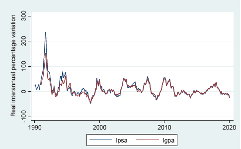
Source: Prepared by the authors based on data supplied by Bloomberg.
Graph 1 Real evolution of stock indexes: January 1990-February 2020.
Following the steps of Lira and Sotz (see Lira and Sotz, 2011), the period up to January 1993 was discarded given the high volatility of the indexes in that period (IPSA reached a value of 236.15% real year-on-year growth while IGPA reached 151.8%).
Proceeding with the data from January 1993, the following series was obtained (the same data only does not consider the period 1990-1993) (see graphic 2).
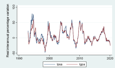
Source: Prepared by the authors based on data supplied by Bloomberg.
Graph 2 Real evolution of stock indexes: January 1993-February 2020.
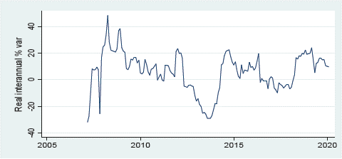
The graph 2 shows that both series follow a similar pattern. It can also be observed that, as of 2012, the series show less volatility compared to previous years.
During the period between January 1993 and February 2020, the real year-on-year percentage change averaged 5.6% and 7.06% for IGPA and IPSA respectively. Contrasting this with the Lira and Sotz data, it can be observed that extending the series for almost 10 years, lower values of inter-annual variation were obtained (compared with the average real inter-annual return for the period January 1993 - May 2010 of 7.5% and 10.2%, for the IGPA and IPSA respectively).
The trend of the IGPA and IPSA series is downward, as the profitability of risky assets has been compressing over the years.
In terms of data volatility, the extended IGPA and IPSA evolution series covering 23 years of data represent slightly lower standard deviations compared to the Lira and Sotz series, which reached 20.2% for IGPA and 22.5% for IPSA in 23 years, different from the 22.1% and 25% for IGPA and IPSA, respectively, obtained by the aforementioned authors. In terms of minimum and maximum values, no changes are observed, which confirms that in recent years the series show less volatility. Maximum real year-on-year return was obtained in May 1994: 79% variation of IPSA. The minimum return reached -47.49% in August 1998, also recorded by IPSA (see table 1):
RISK FREE RATES
For risk-free rates, two series of different durations were constructed from Central Bank and Treasury instruments: 1 and 5 years. The one-year risk-free rate (TLR1) was constructed based on month-end bids of 360-day Central Bank Discount Notes (PDBC) between March 1998 and October 2019 (see graphic 3). The values were brought to real terms using the inflation of the last 12 months calculated according to UF. The series consists of 101 observations over almost 22 years. The average real return of the PDBCs reaches 2.84%, with a standard deviation of 3.86%, a minimum of -9.20% and a maximum of 12.32%. The TLR1 series constructed for the purposes of this paper differs from the Lira and Sotz series (see Lira and Sotz, 2011): the average real return is somewhat lower compared to the original series (2.84% vs. 3.5%), standard deviation is slightly higher (3.86% vs. 3.4%). The TLR1 series of Lira and Sotz has a minimum at -3.6% and a maximum at 14%.
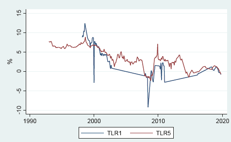
Source: Prepared by the authors based on data supplied by Central Bank and INE.
Graph 3 Real evolution of risk-free rates January 1992-February 2020.
The differences between the series are due to the following reasons: the TLR1 series described in this paper only contains data from PDBC bids, while the Lira and Sotz series is constructed from PDBCs and the Chilean Central Bank's Adjustable Paddles (PRBC). The latter data corresponding to the PRBC are no longer available in the Central Bank's web page, therefore, they could not be used for the construction of the TLR1 series. Then, when extending the series for 10 years, again a somewhat lower return is obtained compared to the original series. As in the case of risky assets, the profitability of risk-free instruments follows a downward trend.
The 5-year risk-free rate (TLR5) is constructed by taking the month-end bid prices of the following instruments: 8-year coupon-bearing inflation indexed notes between January 1993 and August 2002; 5-year Peso denominated Central Bank of Chile Bonds between September 2002 and June 2009; 5-year Peso denominated Treasury Bonds and 5-year inflation indexed Treasury Bonds for the period bet-ween July 2009 and October 2019. The prices of Central Bank and Treasury 5-year peso bids were converted to real terms using inflation of the last 12 months. For the months between July 2009 and October 2019 where both Treasury Bonds and Central Bank Bonds were tendered, a weighted average was calculated to obtain a 5-year risk-free instrument yield.
The TLR5 series consists of 262 observations over almost 27 years. Average real return reaches 3.95%, lower compared to the 4.7% return of the Lira and Sotz series (see Lira and Sotz, 2011), has a standard deviation of 2.52%, somewhat higher than the 2 % of the Lira and Sotz series (see Lira and Sotz, 2011), minimum at -2.35% and maximum at 8.8% versus minimum at 1.8% and maximum at 8.8% in the original series. Again, the series has a downward trend (see table 2).
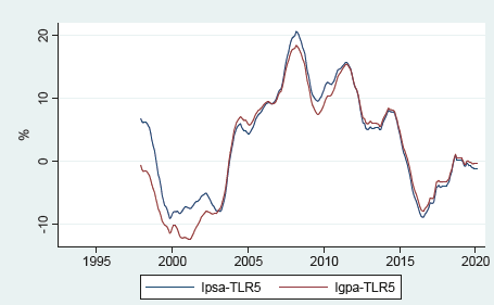
RESULTS: RISK PREMIUM
The actual risk premiums obtained in periods between January 1993 - October 2019 (occupying TLR5) and between March 1998 and October 2019 (occupying TLR1) fluctuate between 1.91% and 4.66% (see graphic 4). When using IGPA, the risk premium totals 2.32% and 2.71% using TLR1 and TLR5, respectively. Calculation based on IPSA gives real risk premium values of 1.91% and 4.66% using TLR1 and TLR5 respectively (see table 3).
Table 3: Real equity risk premiums
| Percentage | ||||
|---|---|---|---|---|
| Average | Standard Deviation | Min | Max | |
| IGPA-TLR1 | 2.32 | 17.88 | -29.86 | 51.69 |
| IGPA-TLR5 | 2.71 | 21.05 | -52.06 | 53.52 |
| IPSA-TLR1 | 1.91 | 18.82 | -30.89 | 50.12 |
| IPSA-TLR5 | 4.66 | 23.42 | -55.61 | 72.59 |
Source: Prepared by the author based on data supplied by Central Bank of Chile and INE.
Comparing with the results published by Lira and Sotz (see Lira and Sotz, 2011), the four series show lower results than the original series. The standard deviations also turned out to be lower in all series compared to the original paper, presenting differences between 6.7% and 1.85% (see table 3).
For the period added in this paper, between June 2010 and October 2019, the risk premium calculated from IGPA reached 4.08% and from IPSA: 3.51%. In the same period, the average real inter-annual return of the stock indexes was 2.87% for IGPA and 2.10% for IPSA. The average real return on 5-year risk-free instruments was 1.77% and 0.36% for 1-year risk-free instruments.
Comparing with the results obtained by the authors in the period between 2010 and 2020, there was an additional decrease in profitability of both risky assets and risk-free assets; consequently, a decrease in risk premium (see graphic 4).
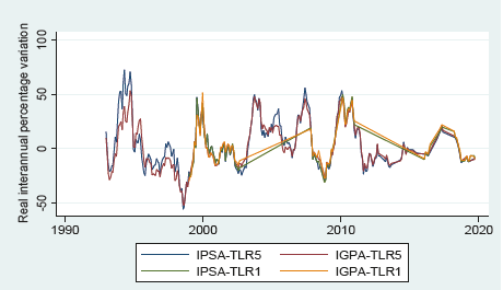
Source: Prepared by the authors based on data supplied by Central Bank, Bloomberg and INE.
Graph 4 Equity risk premium evolution January 1993-October 2019
Following the steps of Lira and Sotz (see Lira and Sotz, 2011) and considering that there are lapses where the average risk premium becomes negative, we proceeded to calculate the moving average risk premium calculated from the 5-year risk-free rate, with a 5-year term window. It was not decided to proceed with risk premium moving averages calculated with 1-year risk-free rate, since that series is much more incomplete.
Considering moving averages of risk premiums calculated from TLR5, it can be seen that the averages turn positive at the end of 2003 and then in mid-2015 they fall back into negative territory, where they are today (see graphic 5).
RISK PREMIUM WITH SECONDARY MARKET DATA
The Central Bank of Chile has data on risk-free rates in the secondary market from September 2002. Since the TLR1 series based on PDBC bid prices is relatively short (101 observations), it was proposed to complement it with secondary market values, using the same methodology to obtain real yield values (see graphic 6).
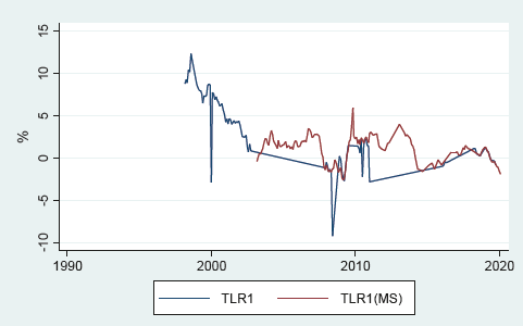
Source: Prepared by the authors based on data supplied by Central Bank.
Graph 6 Real evolution 1-year risk-free rates from primary and secondary markets March 1998-February 2020.
The alternative 1-year risk-free rate series was constructed with data from the primary market (TLR1) and secondary market: (TLR1(MS)). In case both data were available in the same month, primary market data were used. It is worth noting that in the months in which the Central Bank of Chile tendered PDBC, the secondary market rates tended to converge with the bidding rates (see graphic 6).
The following graph shows how both series complement each other, following the same downward trend and converging at points where both data are available.
The series constructed from PDBC bid prices and secondary market securities totals 203 observations, with an average real return of 1.87% (almost one percentage point below the TLR1 average constructed only from primary market bids, 2.84%).
The risk premium rates calculated from the 1-year risk-free rate constructed with primary and secondary market values amount to 7.12% and 7.37% for IGPA and IPSA respectively; 4.8% and 5.46% above risk premiums calculated only from the primary market.
The difference generated is quite significant. Putting together the year-on-year returns of the stock market indexes and the 1-year risk-free instrument rates in graph 7, three time lapses can be highlighted where secondary market data is available and no or very little primary market data is available. These time periods also show relatively high returns on stock market indexes, which leads to a relatively high difference between stock market returns and risk-free asset returns in these periods, significantly increasing the average risk premium calculated from the blended series.
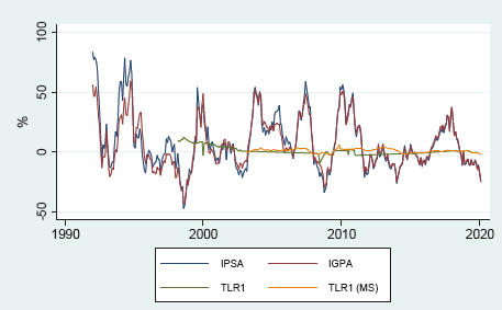
Source: Prepared by the authors based on data supplied by Central Bank, Bloomberg and INE.
Graph 7 Real evolution 1-year risk-free rates in the secondary market and interannual IGPA and IPSA return 1993-February 2020.
The average year-on-year return of stock indexes in months where PDBC was tendered is 2.78% for IGPA and 2.6% for IPSA, while the average year-on-year return of stock indexes in months where only secondary market rates are available, amounts to 12.75% and 13.59%. A possible explanation could be the following: in months marked by high stock market returns, the demand for risk-free paper tends to be lower, which leads prices for risk-free assets to fall (their rates rise) to levels at which the Central Bank does not consider convenient to sell instruments.
Finally, an exercise was also carried out to calculate risk premiums based solely on data from the secondary market between September 2002 and February 2020. For this calculation, we used data of risk-free rates of duration 1 and 5 and, as in previous calculations, real inter-annual returns of IGPA and IPSA stock market indexes. The risk premiums calculated only from risk-free rates in the secondary market are even higher compared to previous calculations. The results were summarized in the following table:
Table 4: Real equity risk premiums
| Percentage | ||||
|---|---|---|---|---|
| Average | Standard Deviation | Min | Max | |
| IGPA-TLR1(MS) | 9.64 | 20.01 | -26.41 | 50.19 |
| IGPA-TLR5(MS) | 6.73 | 19.26 | -31.40 | 49.52 |
| IPSA-TLR1(MS) | 10.05 | 21.84 | -29.89 | 56.41 |
| IPSA-TLR5(MS) | 6.84 | 20.87 | -35.05 | 56.16 |
Source: Prepared by the author based on data supplied by Central Bank of Chile and INE.
IMPLIED EQUITY PREMIUMS
Sources of information and description of the series
In order to estimate the risk premium based on the risk implicit in current stock prices, we seek to construct a dividend yield series. This series consists of the sum of the aggregate dividends of the last 12 months of the stocks included in a given index (in this case IPSA) divided by the market capitalization of the index. The aforementioned series is available on Bloomberg as of March 2006. The series fluctuates between values of 1.53% and 4.15% and averages 2.73%. The series has an upward trend. Compared to the Lira and Sotz series which spans years between 1995 and 2010 and is of similar length, dividend yields have declined over the last few years. The Lira and Sotz series averaged 3.4% and ranged from 1.96% to 7.29% (see graphic 8).
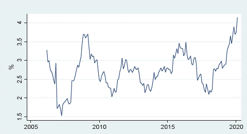
An attempt was made to reconstruct this series with the objective of extending it back to 1995, however, this was not possible. Although it is possible to reconstruct the IPSA indexes composition back to 2001 with data from the electronic Stock Market Information Center, the data corresponding to dividends and market capitalizations are not available for all the companies included in the index at any given time. Therefore, we proceeded only with the aforementioned dividend yield series available in Bloomberg (see graphic 9).
Source: Prepared by the authors based on data supplied by Bloomberg.
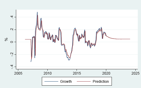
Graph 9 Dividend real growth rate calculated: March 2007-February 2020.
From the dividend yield series, dividends can be obtained by simply multi-plying the dividend yields with the IPSA value in a given month. The dividend series is then translated into real terms using the UF deflector and priced as of the end of February 2020.
The average real year-on-year growth of dividends totaled 5.97% during the period under study and shows a decreasing trend. It can be observed that over the years the growth of dividends has been decreasing. According to Lira and Sotz (see Lira and Sotz, 2011), the average dividend growth rate between 1996 and 2010 (excluding the periods of time when dividend yield reached maximum values) averaged 6.7% and showed a significant stabilization after 2006. In the series presented in this paper covering the years 2007 - 2020, we can see that values have continued to stabilize (compared to data from the late 1990s and early 2000s) and that real returns on risky assets have declined (see graphic 9).
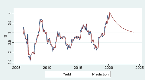
The dividend yield projection was made based on an ARIMA (1,0,1) model, a statistical model used to estimate the temporal dynamics of a time series. This model was chosen considering the importance of the last dividend in the total effect and the previous moving average.
According to the model applied to the dividend yield series, the predicted value for 12 months between March 2020 and February 2021 was 3.79%, above the historical average of 2.73%. The model used and the graphical projection of the results are shown in Table 5 and Graph 10. (Excel method 2 calculation, same series as the previous graph).
Table 5 The model used and the graphical projection.
| Variables | (1) Yield | (2) ARMA | (3) Sigma |
|---|---|---|---|
| L.ar | 0.952*** (0.0292) | ||
| L.ma | -0.0927 (0.0870) | -9.20 | |
| Constant | 2.912*** (0.304) | 0.190*** (0.00725) | |
| Observations | 168 | 168 | 168 |
Source: Prepared by the authors (Standard errors in parentheses ***p< 0.01, **p<0.05, *p<0.1).
Source: Historical data based on Bloomberg, and projections prepared by the author's.
Graph 10 Dividend Yield.
The projection of dividend growth was made on the series of real year-on-year dividend growth between March 2007 and February 2020. The model used to estimate year-on-year real dividend growth was again the ARIMA (1,0,1) model. The projected result was 7.01% for the 12 months between March 2020 and February 2021, slightly above the historical average of 5.97%. The model used and the graphical projection of the results are shown in Table 6 and graphic 11.
Table 6 The model used and the graphical projection.
| Variables | (1) Yield | (2) ARMA | (3) Sigma |
|---|---|---|---|
| L.ar | 0.8832*** (0.0383) | ||
| L.ma | 0.00656 (0.0595) | ||
| Constant | 2.912*** (0.304) | 0.0725*** (0.00240) | |
| Observations | 156 | 156 | 156 |
Source: Prepared by the authors (Standard errors in parentheses ***p< 0.01, **p<0.05, *p<0.1).
CALCULATION OF STOCK RETURN AND RISK PREMIUM
Based on the regressions performed, a projected stock return of 10.8% (3.79% projected dividend yield + 7.01% projected dividend growth) is obtained. The result obtained is somewhat above IPSA's average real year-on-year return of 7.06%.
Subtracting the risk-free rate from the projected stock return, we obtain a risk-free rate of 6.85% (if the 5-year historical average risk-free rate is used), 10.28% if the 5-year average risk-free rate of the last 12 months (March 2019 - February 2020) is used, and 7.96% if the 1-year historical average risk-free rate is used (see table 7).
Table 7 Real equity risk premiums.
| Percentage | |
|---|---|
| Dividen Yield Real dividend growth rate Stock return |
3.79 7.01 10.8 |
| Historical TLR1 Historical TLR5 Last 12 months TLR5 |
2.84 3.95 0.52 |
| Equity risk-premium RA-Historical TLR1 RA-Historical TLR5 RA-Last 12 months TLR5 |
7.96 6.85 10.28 |
Source: Prepared by the authors based on data supplied by Central Bank of Chile and INE.
ADDITION OF THE COUNTRY RISK PREMIUM TO THE RISK PREMIUM OF MATURE ECONOMIES.
Considering that risk premiums in developed economies are lower than in emerging economies, it is possible to deduct a developing economy risk premium by adding a country risk premium to the equity risk premium of a selected mature economy.
For the purposes of this paper and following Damodaran's methodology, the U.S. economy was chosen as a developed economy. Two indicators were then considered: U.S. risk premium calculated from the historical approach and from the implied equity premium approach.
The first indicator was calculated using the Standard & Poor's 500 index as the risky asset and the 10-year U.S. Treasury Bond yield as the risk-free asset. The S&P 500 data are available in Bloomberg from April 1981, which allows us to have real year-on-year return data from April 1982. The constructed series consists of 456 observations over 38 years and delivers average risk premium for the U.S. economy at levels of 4.45% with a standard deviation of 15.94%.
The U.S. economy risk premium based on implied equity premium is published and updated by Damodaran (Damodaran Online) and in February 2020 was equal to 5.2%.
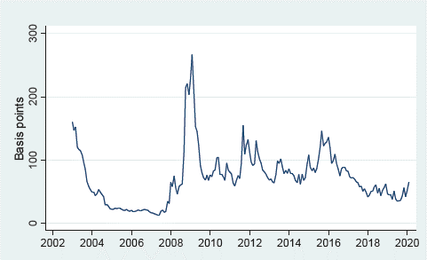
As for the developing economy risk premium, the available country risk measure is Credit Default Swap (CDS), a credit derivative used to hedge the risk of default on a financial asset, a bond or loan in this case. A company's CDS spread is negatively related to its credit rating: the worse the credit rating, the higher the CDS spread. However, there is a large variation in the CDS spreads observed for companies with a given credit rating. The risk of using CDS securities is that they can sometimes be influenced by speculative motives.
Chile's CDS are available in Bloomberg as of January 2003 and show an average of 72.64 basis points (bp) with standard deviation of 42.92 bp (see table 8). While the average presented in this paper is very similar to the Lira and Sotz average of 73.8 bp (see Lira and Sotz, 2011), the series presented here is characterized by less standard deviation (42.92 bp for series between January 2003 and February 2020 vs. 61.8 bp for series between October 2004 and May 2010) (see graphic 12).
Table 8 Real premium in Chile based on USA data and Country risk.
| Percentage | ||
|---|---|---|
| Risk premium in USA | 4.451 | 5.202 |
| Risk premium Chile according to CDS(bp) | 72.64 | 72.64 |
| Risk premium of stock market in Chile | 5.18 | 5.93 |
(1) Estimated on the basis of historical differential returns.
(2) Estimated on the basis of implicit return of stock prices.
Source: Prepared by the authors based on data supplied by Blomberg and Damodaran Online.
Source: Prepared by the authors based on data supplied by Bloomberg.
Graph 12 Credit Default Swap Chile: January 2003 - February 2020.
Calculating Chile's risk premium based on the U.S. risk premium yields measurements that fluctuate between 5.18% - if the U.S. economy risk premium is calculated based on the historical premium approach - and 5.93% if the U.S. economy risk premium is calculated based on the implied equity premium.
CONCLUSIONS
In financial markets dominated by risk-averse investors, riskier assets are priced to appropriately reflect the highest expected return appropriate to the amount of risk assumed. The return above the risk-free rate demanded by investors to hold the portfolio is called the risk premium.
The financial market in Chile has been deepening over the years and currently market capitalization reaches around 84% of GDP, a number that has been declining over the last decade from its peak of 156% in 2010. The last 10 years are also characterized by greater stabilization and an evident downward trend in yields of financial instruments in Chile. Having 10 additional years of history, and therefore a larger amount of data, allows us to estimate the risk premium for the Chilean economy and compare the results with those published by the Central Bank in 2011.
The risk premium in Chile was estimated from three different methodologies and estimates were obtained between 1.91% and 10.28%, depending on the methodology used, which evidences the existence of a positive risk premium of around 5.3%.
Using the historical premium approach in the period between January 1993 and October 2019, the risk premium totaled between 1.91% and 4.66%, depending on the stock index chosen and the risk free rate measure used. It is worth mentioning that, using this method, the results were lower than those found by Lira and Sotz. In addition, it was found that extending the data series allowed to decrease the standard deviation of the series. This turned out to be true both for IPSA and IGPA series and for calculated risk premium series. It has also been observed that, by choosing one or the other stock market index, the results change: in this case the results of risk premium from IGPA show lower average and shorter time span (2.32% and 2.71% versus 1.91% and 4.66% if risk premiums were calculated from IPSA). Results obtained from IPSA are also characterized by higher average premiums. It was also observed that, substituting risk-free rate series from the primary market for the secondary market series, the estimated risk premium is 8.3% on average. The difference generated can be explained by the relationship between fixed income and stock market prices which tend to be in opposite directions. When stock indexes show high yields, appetite for risk-free assets decreases, and paper is not sold because the sale prices are not convenient. By using secondary market rates, no distinction is made between bullish and bearish stock market periods, then it is possible to measure the risk premium in any period.
Following the calculation with the implied equity premium methodology, we obtained a projected stock return of around 10.8% (very similar to that found at the time by Lira and Sotz) and a risk premium between 6.85% and 10.28%, above the results obtained with methods that use only historical data. The results found were also higher than those found by Lira and Sotz using the same method. While in both papers the return projections for stock indexes are quite similar (9.6% in Lira and Sotz's paper vs. 10.8% here), the return on risk-free instruments has declined substantially in recent years. It is also worth noting that Lira and Sotz's projection of returns on risky assets was over 2% higher compared to the actual data. While Lira and Sotz projected stock returns of 9.6%, the actual result was 7.56%. Finally, compared to other calculation methods, only this method resulted in higher risk premiums compared to Lira and Sotz's work. Using differential returns and the risk premium method based on developed economies, lower results were obtained. Using the method of adding country risk premium to the developed economy risk premium, values of 5.18% and 5.93% are found, depending on the chosen method of calculating the U.S. risk premium, and as mentioned above, the risk premium computed with this method has compressed compared to the 2010 result.
In the last 20 years the Chilean economy has faced periods of recession that in comparison with other economies has been different, for example in 2009 there was an imbalance in the financial market in the United States and Europe impacting global growth negatively, however, Chile has been able to respond efficiently and safely to these scenarios. This has had an impact on the series of calculations made to estimate country risk in periods of global uncertainty, attracting emerging economies such as Chile investors protecting their assets. As the calculations consider a number of variables, the results differ from one calculation to another. For example, the calculation of the yield spread considers risk-free financial instruments such as Chile's central bank instruments, as opposed to the calculation of implied return on equity prices, assuming that equity prices are fair, while the third model, Addition to Country Risk Premium, uses the risk premium of the U.S. equity market.
Clearly, the differences are the result of using different variables in different equations, considering that the Chilean economy is classified as an emerging economy and therefore investors will want to obtain higher returns from stocks or financial instruments, the behavior over the last 10 years has tended to stabilize.

