


 Inglês (pdf)
 Artigo em XML
 Referências do artigo
 Enviar este artigo por email
 Citado por SciELO
  Citado por Google
  Similares em
SciELO
Similares em
SciELO  Similares em Google
 Permalink
INTRODUCTION
Contagious COVID-19 illness was initially discovered in late 2019 in Wuhan, China. The World Health Organization (WHO) proclaimed it a global pandemic and the century's worst catastrophe in March 2020 (Baek et al., 2020). The issue has had far-reaching consequences that go beyond health. Closure/lockdown of countries transmit a higher economic cost, and it has become an issue of life against livelihood (Bakhshi & Chaudhary, 2020; Papadamou et al., 2020). The economy's profitability has resulted in a negative stock market. The stock market's feel-good factor is a significant indicator of the future return of a country's capital market. This moment of self-effect rapidly transforms into a concerning factor for shareholders during a crisis, resulting in a negative market with no change in company fundamentals (Just & Echaust, 2020). Thus, analyzing the stock market during a crisis period when security fundamentals are diluted by macroeconomic variables is a significant problem, which is magnified in any open economy when the financial crisis is caused by a pandemic (Sadiq et al., 2021). Uncertainty and risk are created as a consequence of the epidemic, which has a significant economic impact on both advanced and rising economies, such as the United States, Spain, Italy, Brazil, and India. In terms of infections and deaths, India was second only to the United States among the worst-affected countries. The financial market has reacted with spectacular movement in this setting and has been negatively impacted. As a result of the worldwide market disruption, India's financial market has seen significant volatility. COVID-19's influence on the Indian stock market has been dubbed a "black swan event" by some economists, referring to the occurrence of a highly unexpected event with devastating results. Like the stock market, the foreign exchange market is widely viewed as a key indicator of the status of a country's financial markets, and the exchange rate-stock price correlation has sparked enormous attention. For example, the S&P 500, DJI Average, and NASDAQ indices in the United States (US) plummeted until the government got Coronavirus Aid. Although all major stock markets reached their lowest point in the COVID-19 financial meltdown in March 2020, the recovery has been patchy. While some markets-like those in the United States-have recovered to reach new highs by the end of 2020, others, such as those in the United Kingdom, have remained below their pre-COVID peaks.
During the first wave of the COVID-19 pandemic, Contessi and De Pace (2021) detected moments of somewhat explosive dynamics and stock market breakdowns in 18 major countries, discovering statistical proof of China's volatility spreading to all other markets. Al-Awadhi et al. (2020) used panel data analysis to investigate the impact of the COVID-19 outbreak on the Chinese stock market, finding that daily increases in total confirmed cases and total mortality cases caused by COVID-19 had a significant negative impact on stock returns across the board. The exposure of stock markets to various hazards, such as the global financial crisis of 2008, which pushed these markets into a melting position, is the fundamental cause of this extreme collapse. Investors' confidence in the stock market has eroded because of the epidemic since market uncertainty was at an all-time high, as COVID-19 has wreaked havoc on the world's financial and commodities markets, economic activity, employment, and GDP. If someone can correctly forecast price volatility in the stock market or commodities market, they may create suitable investing methods and make better profits (Sharma, 2020). Because it aids investors in risk management, derivative pricing, hedging, and price prediction, the measurement of volatility has a variety of uses in the stock and commodities markets, particularly in trading, investing, and portfolio selection (Li et al., 2020). Furthermore, understanding volatility allows for forecasting the direction of any market, and everyone may have a decent idea of what to expect from the economy; therefore, volatility has applications outside the stock and commodity markets (Chaudhary et al., 2020). In this case, the financial market of India has witnessed sharp volatility resulting from the disruption of the global market. After the COVID-19 outbreak, the stock market came under fear, as BSE Sensex and NSE NIFTY fell by 38%. It led to a 27.31% loss in the total stock market from the beginning of this year (Ambros et al., 2021). Many algorithmic functions for modelling volatility-including autoregressive conditional heteroscedasticity (ARCH), generalized autoregressive conditional heteroskedasticity (GARCH), exponential generalized autoregressive conditional heteroskedasticity (EGARCH), and threshold autoregressive conditional heteroskedasticity (TARCH)-are employed in current approaches. These volatility models are used to explain a changing, potentially volatile variance and forecast the volatility of time series data (Iqbal et al., 2010; Li et al., 2021). In contrast, the "stock-orientated" approach asserts that the exchange rate adjusts to equate the demand and supply of alternative financial as-sets, including domestic money, domestic bonds and equities, and foreign securities.
One of the primary reasons for market integration is the movement of financial crises between various markets. Over the last few decades, knowledge of financial information overflowing from one market to another has gotten a great deal of attention (Bora & Basistha, 2021). The principal goal of researchers is to offer insights regarding market integration since two integrated markets will not provide portfolio diversification advantages. In various countries, much research has observed the information spillover between the two financial markets (foreign exchange and stock market) (Wei et al., 2020). Most research has focused on volatility transmission between foreign exchange and the stock market. Most researchers have focused on industrialized nations (Si et al., 2021), and academics have looked at volatility spillover effects in developed equity markets; however, some studies have examined both developing and emerging equity markets (Purankar & Singh, 2020). The second line of investigation into bond market evolution is from the standpoint of a stock-bond interdependence paradigm. These studies look at topics like comovement between equity and bond markets across emerging economies, with a particular focus on risk segmentation (Faniband & Faniband, 2021), the impact of sovereign credit risk ratings on equity bond relationships, bond with equity within a portfolio consideration, and how interest rate shocks affect bond markets (Roy & Roy, 2017).
Contributions of the study
This article combines India's equity and bond index markets to assess the volatility and spillover impact before and during COVID-19.
This study attempts to interpret the impact of COVID-19 on the Indian stock market, as India is one of the most rapidly transforming engines of the growing economy.
The novel coronavirus has emerged as a popular topic for academics to investigate, posing significant challenges for economic and financial sustainability. Few studies, however, have explored this direction, studying the influence of COVID-19 volatility and spillover effects on the NSE stock exchange and sectoral indices, as well as comparing the bond index to the Indian equities market.
Consequently, the article utilized the daily closing prices of the NSE stock exchange (NIFTY 50 and NIFTY 500) and four NSE sectoral indices (Bank, Auto, IT, Pharma) from September 8, 2019, to July 9, 2021. Initially, the threshold generalized autoregressive conditional heteroscedasticity (TGARCH) model (1,1) was utilized to evaluate the volatility and return of NSE-listed shares.
Secondly, it compared stock market returns with worldwide indices, such as Nikkie225, NASDAQ, and the FTSE100. This time frame was chosen to include both the pre-COVID (September 8, 2019, to December 31, 2019) and the COVID period (January 1, 2020, to July 7, 2021).
The study used the VAR-BEKK-GARCH model to explore the volatility spillover influence on the India-NASDAQ bond index.
The rest of the paper is laid out as follows. Section 2 presents the current literature on COVID-19 and its influence on stock market volatility performance. Section 3 describes the effects of COVID-19 in India, while Section 4 explains the methodological framework. The results and findings are discussed in Section 5, and, finally, Section 6 draws conclusions with some policy implications.
THEORETICAL BACKGROUND AND LITERATURE REVIEW
Many empirical research studies in advanced and emerging nations have looked at the influence of COVID-19 on the financial and stock markets. In this regard, the existing literature has yielded a variety of results. This section summarizes available research findings on the association between pandemics and financial markets. Limited research has been done on the impact of COVID-19 and its unexpected outcomes on stock and sectoral market volatility spillover based on COVID infected and non-infected stages. Gupta et al. (2022) examined the influence of new COVID-19 on the returns and volatility of Indian stock markets, focusing on the Bombay Stock Exchange's equity investing methods, observing the period from March 2015 to January 2021. Pre-estimation tests (Augmented Dickey-Fuller and ARCH-Lagrange multiplier) were performed before applying the GARCH model. The outcomes evidenced that all the strategy indices had negative returns throughout the crisis, implying that the COVID-19 outbreak resulted in huge losses. However, the study is limited to the Indian economy and BSE's stock investment techniques. Sectoral or overall market analysis may be more thorough, providing information on the volatility of each sector during the epidemic.
With the aid of a GARCH model, Bora and Basistha (2021) experimentally explored the influence of COVID-19 on the volatility of stock prices in India. Using daily closing prices of stock indices, NIFTY, and Sensex, from September 3, 2019, to July 10, 2020, the authors sought to compare stock price returns in pre-COVID and post-COVID-19 scenarios. According to the findings, the stock market in India witnessed volatility throughout the epidemic. When comparing results from the COVID era to the pre-COVID period, the study discovered that returns on the indices were larger in the pre-COVID than in the COVID-19 period. However, there is a gap in the study's research on volatility in sectoral indices. Later, Bal and Mohanty (2021) investigated the linear and nonlinear association between daily verified COVID-19 cases and stock market volatility in India's various sectors. Bidirectional causality was revealed using the linear Granger causality test. Furthermore, the study found that stock market volatility and COVID-19 have bidirectional nonlinear Granger causality. This means that previous and lagged data can help forecast COVID-19 instances and the stock market. The results are not sensitive and are consistent in general.
Rakshit and Neog (2021) explored the impact of exchange rate volatility, oil price returns, and COVID-19 instances on stock market returns and volatility for a group of emerging market nations. In addition, their research compared developing market performance during the COVID-19 pandemic to pre-COVID and the Global Financial Crisis (GFC) periods. The authors' findings showed that currency rate volatility had a negative and considerable impact on market returns in Brazil (BOVESPA), Chile (S&P CLX IPSA), India (SENSEX), Mexico (S&P BMV IPC), and Russia (MOEX). As for the impact of oil price returns, the authors found a positive correlation between oil price and stock market returns in all the economies studied. During the epidemic, stock market returns in the selected emerging economies became extremely erratic. Similarly, Guru and Das (2021) examined the influence of COVID-19 on volatility spillovers among ten key sector indices listed on the BSE India. They discovered that overall volatility spillovers reached 69% during COVID-19. The biggest net volatility transmitters were the energy industry, followed by oil and gas. This study aids investors and portfolio managers in assessing risk based on the dynamics of spillovers and in making decisions about asset allocation and portfolio diversification. Stocks from weakly linked industries can help investors limit their exposure to extended uncertainty by incorporating them into their portfolios. The findings revealed that multiple shocks occurred during the study period, but COVID-19 caused the most uncertainty. Volatility spillovers appear to be bursting, implying that shocks travel freely and fast among highly interconnected sectors.
Accordingly, Malik et al. (2021) suggested the GARCH model under diagonal parameterization, used to estimate the multivariate GARCH framework, also known as the BEKK model, on stock market returns of BRIC nations and the US. The empirical results demonstrate that the model captures volatility spillovers and has statistical significance for both short- and long-run persistence effects for its own historical mean and volatility. In addition, given a dynamic framework, it is possible to expand the study to include other rising market economies. Bharti and Kumar (2021) reported market-wide herding behavior in the Indian stock market during the propagation of the COVID-19 outbreak, also investigating the influence of market volatility and government reaction on herding in the research period. For the S&P CNX NIFTY Index and its 50 component businesses, they used the cross-sectional absolute deviation measure and semiparametric estimator of quantile regression for the period January 1, 2020, to June 15, 2020. The findings show substantial herding in the Indian stock market, which gets exacerbated by market volatility. Furthermore, they demonstrate that the government's reaction and control measures are effective in curbing herd behavior. The report suggests implementing higher information disclosure standards to improve market efficiency.
Rai and Garg (2021) analyzed the impact of the COVID-19 pandemic on dynamic correlations and volatility spillovers between stock prices and currency rates in BRIICS economies. Using volatility modeling, the study showed high volatility spillovers and negative dynamic correlations between stock and exchange performance in important BRIICS economies. Moreover, throughout the early days of lockdowns, the bond grew stronger. The findings are solid since they passed the sensitivity analysis. Overall, the data suggest that during the COVID-19 epidemic, there were large risk transfers between the two markets, resulting in a drop in domestic stock returns and in subsequent capital outflows, and rising exchange rates. Safwan (2022) used risk-adjusted return metrics to examine the performance of NSE sectoral indices during the COVID-19 pandemic period. In every performance metric, the pharmaceutical industry beat all others, while real estate, media, and financial services underperformed. Because the financial services sector accounts for 33% of the NIFTY 50, its performance significantly affected the behavior of the index. The financial services, energy, gas, and information technology sectors had a greater impact on the benchmark index. This study focused solely on the effect of the sector market on the COVID-19 period.
Safitri (2022) investigated the influence or impact of the black swan event (COVID-19) on the value of IHSG and Sectoral Index on the IDX, as well as the magnitude of the change in this value before and after COVID-19. The IDX Sectoral Indices and all IHSG values were used as samples in this investigation, which applied Structural Equation Modeling (SEM) with the WarpPLS approach and the Wilcoxon signed-rank test as analytical tools. The Black Swan Event had a negative and significant effect on the movement of the IHSG, according to the analytical results employing SEM with the WarpPLS technique. Investors will also require more profound research to deal with this black swan event.
To address the mentioned challenges, the present research examines the volatility performance of the NSE stock exchange and sectoral indices during and before the COVID-19 pandemic, as well as compares the Indian equities market to the bond index for spillover analysis on the NSE benchmark index. The study also aims to make investment recommendations during times of crisis by identifying the best-performing sectors in terms of risk-adjusted returns.
IMPACTS OF THE PANDEMIC ON INDIAN STOCK MARKETS
Several academics have delved specifically into the Indian stock market. Alam et al. (2020b) used a random sample of 31 businesses listed on the BSE to research the Indian stock markets. Employing the event study technique, the authors examined market reaction during the lockdown period. Despite previous negative returns, stock markets produced positive returns after the lockdown was initiated. With panic spreading through the world beginning in January, the Indian stock markets dutifully responded by falling, and investors welcomed the government's lockup, as evidenced by high returns. Using the Markov-switching vector autoregression, Mishra et al. (2020) demonstrated negative growth in the Indian stock market during the pandemic phase. Except for the pharmaceutical industry, the analysis of other indices yielded the same conclusions. Even the consumer products industry was less damaged than other industries, like metal, real estate, finance, and autos. The authors compared the findings to two previous events-the installation of GST and the implementation of demonetisation-and concluded that none had such a significant influence on the stock markets. COVID-19 has a detrimental effect on returns, according to Bora and Basistha's (2020) research. They also found higher volatility in the stock markets after the first COVID-19 instance was announced, using data from both BSE and NSE. Rajamohan et al. (2020) found similar results while examining stock price volatility in the Indian car sector. COVID-19 cases had little impact on the volatility of the Indian stock markets and did not affect returns, according to Verma and Sinha (2020). These findings may be due to the study's timing, as it was conducted during the early stages of COVID-19 dissemination in India (in May 2020).
PROPOSED RESEARCH METHODOLOGY
Following the recent COVID-19 epidemic, stock markets worldwide experienced varying levels of volatility. As explained, this article examined the impact of the pandemic on stock market volatility and spillover from the NSE's Indian stock market to the international stock market. It suggests the influence of COVID-19 on the performance of the Indian stock market using two composite indices (NIFTY 50 and NIFTY 500) and four NSE sectoral indices (Bank, Auto, IT, Pharma), aiming to calculate daily stock market returns and volatility. The study used the TGARCH model (1,1) to investigate the volatility of NSE traded shares. The daily return series' conditional volatility indicates volatility changes across the study period. This research compares India's composite indices to three worldwide indices: Nikkei 225, NASDAQ, and FTSE100, during the COVID-19 period from September 8, 2019, to July 10, 2021.
The proposed work's architecture is depicted in Figure 1. This article aims to investigate the impact of volatility spillovers between foreign exchange and stock market in India during the pre-COVID and COVID periods. Given that the research specifies the positive definite covariance matrix, the multivariate GARCH with the BEKK specification established by Engle and Kroner (1995) appears to be well suited to examine volatility spillover effects. This finding might aid investors, politicians, and portfolio managers in making sound investment decisions. The impact of two events (included in the study) that may have impacted India's bank stock indices has been investigated and compared using volatility models. Initially, a descriptive analysis using mean, standard deviation, skewness, kurtosis, and the Jarque-Bera statistic was employed to understand data properties for all three variables. The conditions for using volatility models have also been examined.
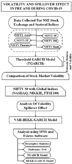
Data collection and market classification
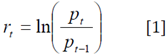
The research used daily pricing data from the Yahoo Finance website on the NIFTY 50 and NIFTY 500 stock market indices, as well as four NSE sectoral indices (Bank, Auto, IT, Pharma) in India, to compare them to worldwide indices, such as Japan's Nikkei 225, the US NASDAQ, and the UK FTSE 100 (FTSE100). The research ran from September 8, 2019, to July 10, 2021. This time frame was chosen to include the pre-COVID (September 8, 2019, to December 31, 2019) and COVID period (January 1, 2020, to July 7, 2021) since this time frame provides a better understanding of stock market behavior. Consequently, the NSE daily stock return series was calculated using the following log transformation,
Where r t is the logarithmic return on DSE indices for time t, p t is the closing price at the time t, and pt1 is the corresponding price in the period at a time t-1. For the quantitative study, the EViews statistics software was employed. The analysis was carried out using unit root test, descriptive statistics, ARCH effect test, and the GARCH model, among other statistical approaches.
Methodology of unit root test estimation
A stationary check is required in this time series analysis. The unit root test is commonly used to determine whether data are stationary. The study used the Augmented Dickey-Fuller (ADF) test and the Kwiatkowski-Phillips-Schmidt-Shin (KPSS) tests in this respect. Volatility is well-known to be represented using the GARCH family of models. Typically, the mean equation is employed to characterize the series' level, while the ARCH model is applied to predict the variance. When data is serially correlated, the mean equation's misspecification may fail to resolve the autocorrelation problem that might develop in the volatility model. Moreover, the precise definition of the mean equation is critical. Therefore, all the GARCH family models were estimated with the following acceptable mean equation as stated below,

To establish the variance equation to represent volatility for various applications, this paper employed TGARCH family models. Changing distributional assumptions were used to test the sensitivity of the model's estimation findings. From a normal distribution to a Student's t-distribution, the distributional assumption is modified. The rationale for this is that it is well documented in many research studies on financial asset returns that the return variable is more likely to follow a "levy distribution" with "fat tails" and that kurtosis is likely to grow as data frequency increases (Andersen & Bollerslev, 1998). The following is an example of a helpful variance equation,
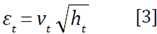
Where v t ~ i.i.d(0,1) and
GARCH model
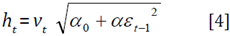
Engle (1982), the founder of volatility modelling, employed the ARCH model. The fundamental issue with this model is that it frequently requires a significant lag to represent time-varying volatility in reality. Bollerslev (1986) introduced the GARCH model, which permits conditional variance to be dependent on its lag, reducing the number of necessary ARCH lags. Subsequently, the conditional variance equation should be:

Here, the GARCH (1,1) model has one ARCH term denoted as E [ _ 1 2 and one GARCH term denoted as h t1 . Some constraints are required for the variance to stay properly behaved (finite and positive) α > 0, α 0 > 0, β > 0. Volatility persists due to the sum of the ARCH and GARCH coefficients. To ensure that series e t is stationary and the variance is well behaved, it is necessary to assume that α + β< 1.
TGARCH model
Zakoian (1994) and Glosten et al. (1995) presented the TGARCH model (1993). The model's specification for the threshold GARCH (1,1) is as follows:

Where  (good news) and ε
t-1
< 0 (bad news) produce a differential effect on the conditional variance. Good news has an impact on a while bad news affect (a +
Y).
When
Y
is significant and positive, volatility is more affected by negative shocks than by positive ones. Here, non-negativity restrictions are also needed for
a, a
0
, Y
and
p
like that of standard GARCH (1,1).
(good news) and ε
t-1
< 0 (bad news) produce a differential effect on the conditional variance. Good news has an impact on a while bad news affect (a +
Y).
When
Y
is significant and positive, volatility is more affected by negative shocks than by positive ones. Here, non-negativity restrictions are also needed for
a, a
0
, Y
and
p
like that of standard GARCH (1,1).
Measuring volatility spillovers using the VAR-BEKK-GARCH model
To assess the returns and volatility spillovers between foreign exchange and stock market, the study employs the Diebold and Yilmaz (2009) spillover index approach. VAR models are used to calculate these spillovers. The VAR model aids in the break-down of prediction error variance, offering a measure of each variable's overall relative relevance in causing changes in its own and other variables. Decomposing this forecast variance allows seeing how each variable in the system affects itself and other variables across different time horizons (e.g., h-step forward). To investigate the impact of the stock market and foreign currency volatility spillovers, the study defines the multivariate GARCH with the BEKK model. The BEKK specification is remarkable given that it does not limit the correlation structure between the variables. The conditional mean equation is simulated using a vector autoregressive (VAR) model for the empirical examination of volatility spillover. The VAR (1) model is chosen based on the notion of minimal Akaike information criterion values, and it may be defined as follows,

Where r t is the returns matrix of the foreign exchange and stock markets; n is a 3 x 1 vector of constant; and μ is a 3 x 1 vector of the residual and follows a normal distribution in which the mean is zero and μ t is the conditional variance-covariance matrix. C is a constant matrix and 3 x 3 lower triangular vector, where the constant c is included. D is a 3 x 3 parameter matrix of conditional variance, where d represents the relation of the conditional variance between market i and market j. A is a 3 x 3 parameter matrix of residual, where a., is included to capture the ARCH effect in the residual in market i and market j. The Wald test was used to assess the volatility spillover effect's null hypothesis, that is, if the difference of A and D equals zero. For market i and j, the Wald test hypothesizes that A(i, j) = D(i, j) = 0. The null hypothesis was rejected, indicating that market risk had spilt over i to j.
A wide range of real-time data may be used to evaluate the research project. For performance analysis, data outputs must be documented and visualized. The following approach may be executed and simulated using SPSS and EViews software; the stock market's performance during COVID-19 is compared to the world stock market for a more accurate comparison.
EXPERIMENTATION AND RESULTS DISCUSSION
The NSE index's daily closing price is non-stationary, so it is turned into a daily logarithmic return series to make the series stationary. This return series has now reached a point of equilibrium (presented later in Figure 8). Figure 2 summarizes the descriptive information on NSE stock return. SPSS and EViews software were used to conduct the analysis. Structural equation modelling, as well as basic descriptive statistics, unit root test, and the GARCH model were employed in the analysis.
Descriptive statistics
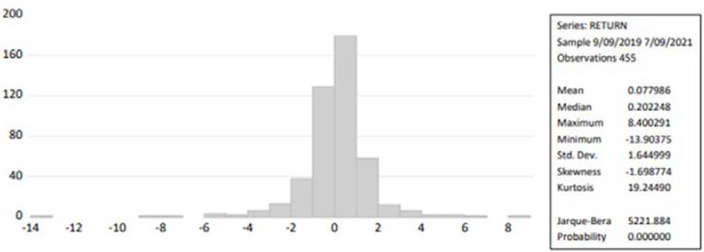
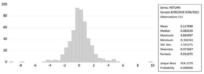
The daily return series of financial assets throughout the research period was evaluated for distributional properties using stock market descriptive statistics. Jarque-Bera probability is used to assess the mean (X), standard deviation (SX), skewness (S), and kurtosis (K) in Figures 2-6.
Figure 2 signposts the descriptive statistics for the NIFTY 50 stock market return value. The average return of the stock market in a day was 7.79% and on the remaining days the return is less than 2.02%. The maximum return in one day was 8.40%, while the minimum loss in a day was -13.90. In the meantime, the standard deviation in the market was 1.644 and the result of the skewness is negative (-1.698), which illustrates that data are negatively skewed, and kurtosis data have improved productivity. In addition, the Jarque-Bera test result value was 5221.884, confirming that the data of variables are not distributed normally.
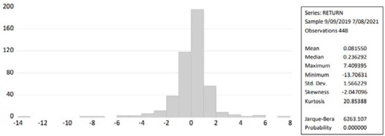
The descriptive statistics for the NIFTY 500 stock market return value are shown in Figure 3. The stock market's average daily return was 8.15%, with returning of less than 3.62% on the remaining days. The greatest daily return was 7.409, while the smallest daily loss was -13.70. While the market's standard deviation was 1.566 and the skewness result was negative (-2.047); this indicates that the data are negatively skewed, and kurtosis data have enhanced productivity. Furthermore, the result of the Jarque-Bera test was 6263.107, indicating that variable values are non-normally distributed.
The descriptive statistics for the NIFTY bank stock market return value are exposed in Figure 4. The stock market's average daily return was 4.50%, with a returning of less than 3.47% on the remaining days. The greatest daily return was 9.9951, with the smallest daily loss being -18.313. The market's standard deviation was 2.346 and the skewness result was negative (-1.162), which indicates that the data are negatively skewed, and kurtosis data have enhanced productivity.
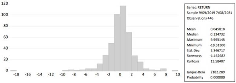
Moreover, the result of the Jarque-Bera test was 2182.289, indicating that variable values are non-normally distributed.
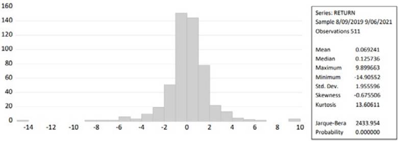
The descriptive statistics for the Nifty auto stock market return value are displayed in Figure 5. The stock market's average daily return was 6.92%, with the returning less than 1.25% on residual days. The highest daily return was 9.899, with the lowest daily loss being -14.905. The market's standard deviation was 1.9555 and the skewness result was negative (-0.6755), which indicates that the data were negatively skewed, and kurtosis data had enhanced productivity. Additionally, the result of the Jarque-Bera test was 2433.954, indicating that the variable values are not regularly distributed
The descriptive statistics for the NIFTY IT stock market return value are shown in Figure 6. The stock market's average daily return was 5.76%, with a returning less than 8.80% on the rest days. The biggest daily return was 8.64 percent, with the least daily loss being -10.06. The market's standard deviation was 1.681 and the skewness result was negative (-0.765), which indicates that the data are negatively skewed, and kurtosis data have enhanced productivity. Furthermore, the Jarque-Bera test result of 1394.441 demonstrates that the variable values are not normally distributed.
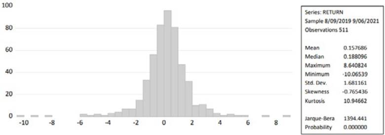
Figure 7 represents the descriptive statistics analysis of NIFTY pharma stock market return values. Given that the skewness and kurtosis of the normal distribution should be 0 and 3, respectively, the mean value of all returns is near zero, and the values of skewness and kurtosis appear to be a deviation from the normal distribution. These figures show that the three markets' returns are characterized by wide tails. The Jarque-Bera test also rejects the null hypothesis, showing that the returns are not distributed normally. These findings support the existence of an ARCH impact on stock prices and market returns
Stock market log-return series
For statistical evaluations like MSPE and out-of-sample R-square, log return is employed. For assessing economic value, such as certainty equivalent return (CER) gain and Sharpe ratio, simple return is employed. This is because for time-series and cross-section viewpoints, respectively, additivity is a property of both log and simple returns. Furthermore, because stock returns are always assumed to follow a log-normal distribution, the log return is utilized for statistical analysis.
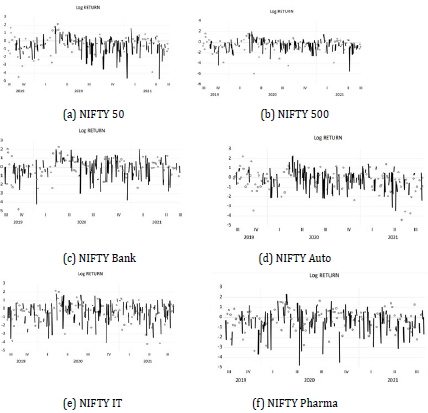
The log returns of the Indian stock indices are revealed in Figure 8. The mean of the log return is anticipated to be virtually zero, but the volatility may increase towards the beginning of 2019 and the beginning of 2020. This occurrence is explained by the adjusted closed price. There are considerable swings in the closure price.
Unit root test using Augmented Dickey-Fuller test
Before running any model, a time series analysis must be carried out for the existence of unit roots. The Augmented Dickey-Fuller test (Cheung & Lai, 1995) was used to determine whether the series was stationary at the level and first difference. Because financial returns are non-stationary, informal testing efficiency with effective fore-casting models may be hampered.
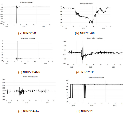
In the regression model of coefficients with the null hypothesis, Figure 9 depicts the unit root test of the ADF analysis. Figure 9(a) states the Dickey-Fuller autoregressive coefficients for NIFTY 50, while Figure 9(b) depicts the same for the NIFTY 500, illustrating the Dickey-Fuller test with the least square support vector regression between from 08-09-2019 to 09-07-2021. Figure 9(c) states the ADF test of NIFTY Bank sectoral indices in the regression model of coefficients with -23.6. Instantaneously, the ADF coefficients for NIFTY IT are shown in Figure 9(d), which are based on a regression model with a 1.909 coefficient in the Durbin-Watson statistic. Figure I(e) and 9(f) illustrate the ADF coefficients for NIFTY Auto and Pharma, respectively. Pharma was tested with the sample R-squared and contained Durbin-Watson statistics with a better coefficient of 2.453.
Test for stationarity using KPSS
To test the stationarity of the return series, unit root tests with breaks were used. To determine stationarity, the KPSS test is utilized. For every return series, the test contradicts the null hypothesis of normality at 1% significance level.
The stationary test for NIFTY 50 is presented in Table 1. The p-value of a test is a probability score that may be used to determine whether the null hypothesis should be rejected. If the p-value is less than a predefined alpha threshold, the null hypothesis is rejected.
Table 1 KPSS Test for Stationary in Nifty 50
|
Null hypothesis: Return is stationary Exogenous: Constant Bandwidth: 12 (Newey-West automatic) using Bartlett Kernel | ||||
| LM-Stat | ||||
| Kwiatkowski-Phillips-Schmidt-Shin (KPSS) test statistics | 0.146520 | |||
| Asymptotic critical values*: | 1% level | 0.739000 | ||
| 5% level | 0.463000 | |||
| 10% level | 0.347000 | |||
| Kwiatkowski-Phillips-Schmidt-Shin (1992, Table 1) | ||||
|
Residual variance (no correction) HAC corrected variance (Bartlett Kernel) |
2.700073 3.081955 |
|||
|
KPSS test equation Dependent variable: RETURN Method: Least squares Date: 10/12/21 Time: 12:50 Sample (adjusted): 9/11/2019 to 7/09/2021 Inclined observations:455 after adjustments | ||||
| Variable | Coefficient | Std. Error | t-Statistic | Prob. |
| C | 0.077986 | 0.077119 | 1.011252 | 0.3124 |
| R-squared | 0.000000 | Mean dependent var. | 0.077986 | |
| Adjusted R-squared | 0.000000 | SD dependent var. | 1.644999 | |
| SE of regression | 1.644999 | Akaike info criterion | 3.835552 | |
| Sum squared resid. | 1228.533 | Schwarz criterion | 3.844607 | |
| Log-likelihood | -871.5880 | Hannan-Quinn criterion | 3.839119 | |
| Durbin-Watson stat. | 2.190281 | |||
Note: * indicates the significance level.
Source: author's elaboration.
The stationary test for NIFTY 500 is depicted in Table 2. The test's p-value is a probability score that may be used to assess whether the null hypothesis should be rejected. If the p-value is less than the current alpha threshold of p=0.2710, the null hypothesis is rejected.
Table 2 KPSS test for stationary in NIFTY 500
| Null hypothesis: Return is stationary Exogenous: Constant Bandwidth: 12 (Newey-West automatic) using Bartlett Kernel | ||||
| LM-Stat | ||||
| Kwiatkowski-Phillips-Schmidt-Shin (KPSS) test statistics | 0.169337 | |||
| Asymptotic critical values*: | 1% level | 0.739000 | ||
| 5% level | 0.463000 | |||
| 10% level | 0.347000 | |||
| Kwiatkowski-Phillips-Schmidt-Shin (1992, Table 1) | ||||
| Residual variance (no correction) HAC corrected variance (Bartlett Kernel) | 2.447597 3.134906 | |||
|
KPSS test equation Dependent variable: RETURN Method: Least squares Date: 10/12/21 Time: 14:02 Sample (adjusted): 8/13/2019 to 9/06/2021 Inclined observations: 511 after adjustments | ||||
| Variable | Coefficient | Std. Error | t-Statistic | Prob. |
| C | 0.081550 | 0.073997 | 1.102062 | 0.2710 |
| R-squared | 0.000000 | Mean dependent var. | 0.081550 | |
| Adjusted R-squared | 0.000000 | SD dependent var. | 1.566229 | |
| SE of regression | 1.566229 | Akaike info criterion | 3.737448 | |
| Sum squared resid. | 1096.523 | Schwarz criterion | 3.746611 | |
| Log-likelihood | -836.1884 | Hannan-Quinn criterion | 3.741060 | |
| Durbin-Watson stat. | 2.164369 | |||
Note: * indicates the significance level.
Source: author's elaboration.
The stationary test for NIFTY Bank is shown in Table 3. The test's p-value is a probability score that may use to decide whether to reject the null hypothesis. The obtained p-value is 0.6856, which is greater than the threshold. Using critical values of 5% for ADF PP and ZA. In the KPSS test, the critical value passes from 1% to 5%, thus it satisfies whether the value is stationary or not. When the differences between the first and second series are added together, the critical value still does not go below 5%.
Table 3 KPSS test for stationary in NIFTY Bank
|
Null hypothesis: Return is stationary Exogenous: Constant Bandwidth: 10 (Newey-West automatic) using Bartlett Kernel | ||||
| LM-Stat | ||||
| Kwiatkowski-Phillips-Schmidt-Shin (KPSS) test statistics | 0.188682 | |||
| Asymptotic critical values*: | 1% level | 0.739000 | ||
| 5% level | 0.463000 | |||
| 10% level | 0.347000 | |||
| Kwiatkowski-Phillips-Schmidt-Shin (1992, Table 1) | ||||
| Residual variance (no correction) HAC corrected variance (Bartlett Kernel) | 5.494734 6.479610 | |||
|
KPSS test equation Dependent variable: RETURN Method: Least squares Date: 10/12/21 Time: 16:17 Sample (adjusted): 9/11/2019 to 7/08/2021 Inclined observations: 446 after adjustments | ||||
| Variable | Coefficient | Std. Error | t-Statistic | t-Statistic Prob. |
| C | 0.045018 | 0.111120 | 0.405131 | 0.6856 |
| R-squared | 0.000000 | Mean dependent var. | 0.045018 | |
| Adjusted R-squared | 0.000000 | SD dependent var. | 2.2346717 | |
| SE of regression | 2.346717 | Akaike info criterion | 4.546151 | |
| Sum squared resid. | 2450.651 | Schwarz criterion | 4.555345 | |
| Log-likelihood | -1012.792 | Hannan-Quinn criterion | 4.549776 | |
| Durbin-Watson stat. | 1.975350 | |||
Note: * indicates the significance level. Source: author's elaboration.
Table 4 KPSS test for stationary in NIFTY Auto
|
Null hypothesis: Return is stationary Exogenous: Constant Bandwidth: 7 (Newey-West automatic) using Bartlett Kernel | ||||
| LM-Stat | ||||
| Kwiatkowski-Phillips-Schmidt-Shin (KPSS) test statistics | 0.117775 | |||
| Asymptotic critical values*: | 1% level | 0.739000 | ||
| 5% level | 0.463000 | |||
| 10% level | 0.347000 | |||
| Kwiatkowski-Phillips-Schmidt-Shin (1992, Table 1) | ||||
| Residual variance (no correction) HAC corrected variance (Bartlett Kernel) | 3.941068 3.816871 | |||
|
KPSS test equation Dependent variable: RETURN Method: Least squares Date: 10/12/21 Time: 13:53 Sample (adjusted): 8/13/2019 to 9/06/2021 Inclined observations: 511 after adjustments | ||||
| Variable | Coefficient | Std. Error | t-Statistic | Prob. |
| C | 0.069241 | 0.086510 | 0.800381 | 0.4239 |
| R-squared | 0.000000 | Mean dependent var. | 0.069241 | |
| Adjusted R-squared | 0.000000 | SD dependent var. | 1.955.596 | |
| SE of regression | 1.955.596 | Akaike info criterion | 4.181.222 | |
| Sum squared resid. | 1.950.421 | Schwarz criterion | 4.189.512 | |
| Log-likelihood | -1.067.302 | Hannan-Quinn criterion | 4.184.472 | |
| Durbin-Watson stat. | 2.076.839 | |||
Table 5 depicts the stationary test for NIFTY IT. The p-value of a test is a probability score that may be used to determine whether the null hypothesis should be rejected. Here, the p-value is less than a predefined alpha threshold, which was p=0.0345, so the null hypothesis is rejected.
Table 5 KPSS test for stationary in NIFTY IT
|
Null hypothesis: Return is stationary Exogenous: Constant Bandwidth: 10 (Newey-West automatic) using Bartlett Kernel | ||||
| LM-Stat | ||||
| Kwiatkowski-Phillips-Schmidt-Shin (KPSS) test statistics | 0.338320 | |||
| Asymptotic critical values*: | 1% level | 0.739000 | ||
| 5% level | 0.463000 | |||
| 10% level | 0.347000 | |||
| Kwiatkowski-Phillips-Schmidt-Shin (1992, Table 1) | ||||
|
Residual variance (no correction) HAC corrected variance (Bartlett Kernel) |
3.816871 3.941068 |
|||
|
KPSS test equation Dependent variable: RETURN Method: Least squares Date: 10/12/21 Time: 13:56 Sample (adjusted): 8/13/2019 to 9/06/2021 Inclined observations: 511 after adjustments | ||||
| Variable | Coefficient | Std. Error | t-Statistic | Prob. |
| C | 0.157686 | 0.086510 | 0.800381 | 0.0345 |
| R-squared | 0.000000 | Mean dependent var. | 0.157686 | |
| Adjusted R-squared | 0.000000 | SD dependent var. | 1.681.161 | |
| SE of regression | 1.681.161 | Akaike info criterion | 3.878.802 | |
| Sum squared resid. | 1.441.415 | Schwarz criterion | 3.887.092 | |
| Log-likelihood | -9.900.339 | Hannan-Quinn criterion | 3.882.052 | |
| Durbin-Watson stat. | 2.217214 | |||
Note: * indicates the significance level. Source: author's elaboration.
Table 6 KPSS test for stationary in NIFTY Pharma
|
Null hypothesis: Return is stationary Exogenous: Constant Bandwidth: 9 (Newey-West automatic) using Bartlett Kernel | ||||
| LM-Stat | ||||
| Kwiatkowski-Phillips-Schmidt-Shin (KPSS) test statistics | 0.043129 | |||
| Asymptotic critical values*: | 1% level | 0.739000 | ||
| 5% level | 0.463000 | |||
| 10% level | 0.347000 | |||
| Kwiatkowski-Phillips-Schmidt-Shin (1992, Table 1) | ||||
|
Residual variance (no correction) HAC corrected variance (Bartlett Kernel) |
2.527202 3.323486 |
|||
|
KPSS test equation Dependent variable: RETURN Method: Least squares Date: 10/12/21 Time: 14:02 Sample (adjusted): 8/13/2019 to 9/06/2021 Inclined observations: 511 after adjustments | ||||
| Variable | Coefficient | Std. Error | t-Statistic | Prob. |
| C | 0.117999 | 0.070394 | 1.676263 | 0.0943 |
| R-squared | 0.000000 | Mean dependent var. | 0.117999 | |
| Adjusted R-squared | 0.000000 | SD dependent var. | 1.591275 | |
| SE of regression | 1.590275 | Akaike info criterion | 3.768904 | |
| Sum squared resid. | 1291.400 | Schwarz criterion | 3.777194 | |
| Log-likelihood | -961.9549 | Hannan-Quinn criterion | 3.772154 | |
| Durbin-Watson stat. | 2.053606 | |||
Note: * indicates the significance level.
Source: author's elaboration.
The presence of a unit root in the return series examined using the KPSS test for NIFTY Pharma is shown in Table 7. The NIFTY Pharma's KPSS test statistic is 0.0943>0.01. Consequently, the null hypothesis is rejected at a 1% significance level. This shows that data had remained static.
Table 7 Estimate result of the TGARCH model for NIFTY 50
|
Dependent variable: NIFTY 50_RETURN Method: ML ARCH-Normal Distribution (BFGS/Marquardt steps) Date:10/13/21 Time: 10:05 Sample: 9/09/2019 to 7/09/2021 Inclined observations: 456 Convergence achieved after 26 iterations Coefficient covariance computed using outer product of gradients Presample variance: backcast (parameter = 0.7) GARCH=C(1) + C(2)*RESID(-1)^2 + C(3)* RESID(-1)^2* (RESID(-1)<0) + C(4)*GARCH(-1) | ||||
| Variable | Coefficient | Std. Error | z-Statistics | Prob. |
| Variance Equation | ||||
| C | 0.051967 | 0.009662 | 5.378212 | 0.0000 |
| RESID (-1)A2 | -0.008336 | 0.012484 | -0.667796 | 0.5043 |
| RESID (-1)A2* RESID | 0.240760 | 0.032463 | 7.416362 | 0.0000 |
| (-1)<GARCH(-1) | 0.864173 | 0.015282 | 56.54688 | 0.0000 |
| R-squared | -0.002263 | Mean dependent var. | 0.078089 | |
| Adjusted R-squared | -0.000065 | SD dependent var. | 1.643191 | |
| SE of regression | 1.643245 | Akaike info criterion | 3.165693 | |
| Sum squared resid. | 1231.316 | Schwarz criterion | 3.201856 | |
| Log-likelihood | -717.7781 | Hannan-Quinn criterion | 3.179938 | |
| Durbin-Watson stat. | 2.185355 | |||
Source: author's elaboration.
The asymmetric influence on the stock index volatility through the COVID period is seen in Table 8. This variance equation features a negative element, which explains why negative returns have more volatility than positive ones. As a result, in the variance equation, the top 50 return values are important. The relationship between the variables is satisfied by the probability p=0, which is less than 0.05.
Table 8 Estimate result of the TGARCH model for NIFTY 500
|
Dependent variable: NIFTY 500_RETURN Method: ML ARCH-Normal Distribution (BFGS/Marquardt steps) Date: 10/13/21 Time: 10:17 Sample: 9/09/2019 to 7/08/2021 Inclined observations: 455 Convergence achieved after 24 iterations Coefficient covariance computed using outer product of gradients Presample variance: backcast (parameter = 0.7) GARCH=C(1) + C(2)*RESID(-1)A2 + C(3)* RESID(-1)A2* (RESID(-1)<0) +v C(4)*GARCH(-1) | ||||
| Variable | Coefficient | Std. Error | z-Statistics | Prob. |
| Variance Equation | ||||
| C | 0.064076 | 0.009644 | 6.644274 | 0.0000 |
| RESID (-1) ^2 | -0.005076 | 0.014646 | -0.346584 | 0.7289 |
| RESID (-1) ^2* RESID (-1)<GARCH(-1) | 0.229690 0.851917 | 0.032624 0.016278 | 7.040637 52.33488 | 0.0000 0.0000 |
| R-squared | -0.003066 | Mean dependent var. | 0.085991 | |
| Adjusted R-squared | -0.000862 | SD dependent var. | 1.554574 | |
| SE of regression | 1.555244 | Akaike info criterion | 3.088611 | |
| Sum squared resid. | 1100.547 | Schwarz criterion | 3.124834 | |
| Log-likelihood | -698.6590 | Hannan-Quinn criterion | 3.102881 | |
| Durbin-Watson stat. | 2.142448 | |||
Source: author's elaboration.
The asymmetric influence on the stock index volatility through the COVID era is depicted in Table 9. The coefficients of the variance equation are represented by coefficients, standard errors, z-statistics, and p-values in the "Variance Equation" section. This variance equation has negative elements, which explains why negative returns have larger volatility than positive ones. As a result, in the variance equation, the top 50 return values are important. The relationship between the variables is satisfied by the probability p=0, which is less than 0.05.
Table 9 Estimate result of the TGARCH model for NIFTY Bank
|
Dependent variable: NIFTY Bank_RETURN Method: ML ARCH-Normal Distribution (BFGS/Marquardt steps) Date: 10/13/21 Time: 9:57 Sample: 9/09/2019 to 7/08/2021 Inclined observations: 455 Convergence achieved after 25 iterations GARCH=C(1) + C(2)*RESID(-1)A2 + C(3)* RESID(-1)A2* (RESID(-1)<0) + C(4)*GARCH(-1) | ||||
| Variable | Coefficient | Std. Error | z-Statistics | Prob. |
| Variance Equation | ||||
| C | 0.082814 | 0.032742 | 2.529301 | 0.0000 |
| RESID (-1) ^2 | -0.036490 | 0.018639 | 1.957742 | 0.0503 |
| RESID (-1) ^2* RESID (-1)<GARCH(-1) | 0.203544 0.856871 | 0.031968 0.022886 | 6.367134 37.44146 | 0.0000 0.0000 |
| R-squared | -0.000650 | Mean dependent var | 0.059279 | |
| Adjusted R-squared | -0.001549 | SD dependentvar | 2.327332 | |
| SE of regression | 2.325529 | Akaike info criterion | 4.076779 | |
| Sum squared resid. | 2460.679 | Schwarz criterion | 4.113002 | |
| Log-likelihood | -923.4673 | Hannan-Quinn criterion | 4.091050 | |
| Durbin-Watson stat. | 1.951670 | |||
Source: author's elaboration.
The asymmetric influence on the stock index's volatility during the COVID period is depicted in Table 10. The coefficients, standard errors, z-statistics, and p-values for the coefficients of the variance equation are all contained in the "Variance Equation" section. The equation's coefficient is negative, implying that negative returns have more volatility than positive ones. Consequently, in the variance equation, the top 50 return values are important. The link between the variables is satisfied when the probability p=0 is smaller than 0.05.
Table 10 Estimate result of the TGARCH model for NIFTY Auto
|
Dependent variable: NIFTY Bank_RETURN Method: ML ARCH-Normal Distribution (BFGS/Marquardt steps) Date: 10/13/21 Time: 9:57 Sample: 9/09/2019 to 7/08/2021 Inclined observations: 455 Convergence achieved after 25 iterations Coefficient covariance computed using outer product of gradients Presample variance: backcast (parameter = 0.7) GARCH=C(1) + C(2)*RESID(-1)^2 + C(3)* RESID(-1)^2* (RESID(-1)<0) + C(4)*GARCH(-1) | ||||
| Variable Coefficient | Std. Error | z-Statistics Prob. | ||
| Variance Equation | ||||
| C | 0.055757 | 0.014426 | 3.865169 | 0.0001 |
| RESID (-1) ^2 | -0.009973 | 0.010171 | -0.980490 | 0.3268 |
| RESID (-1) ^2* RESID (-1)<GARCH(-1) | 0.137330 0.921740 | 0.018479 0.013896 | 7.431600 66.32949 | 0.0000 0.0000 |
| R-squared | -0.001008 | Mean dependent var. | 0.062181 | |
| Adjusted R-squared | -0.000947 | SD dependent var. | 1.960202 | |
| SE of regression | 1.959273 | Akaike info criterion | 3.781535 | |
| Sum squared resid. | 1965.441 | Schwarz criterion | 3.814647 | |
| Log-likelihood | -964.0729 | Hannan-Quinn criterion | 3.794514 | |
| Durbin-Watson stat. | 2.061085 | |||
Source: author's elaboration.
Table 11 illustrates the asymmetric effect on the volatility of the stock index during the COVID period. This contains the coefficients, standard errors, z-statistics, and p-values for the coefficients of the variance equation. The coefficient of the equation is negative; this gives higher volatility as compared to the positive returns. Correspondingly, the NIFTY 50 return values are significant in the variance equation. The probability p=0, which is less than 0.05, thus satisfying the relation between the variables.
Table 11 Estimate result of the TGARCH model for NIFTY IT
|
Dependent variable: NIFTY IT_RETURN Method: ML ARCH-Normal Distribution (BFGS/Marquardt steps) Date: 10/13/21 Time: 10:12 Sample: 8/09/2019 to 9/06/2021 Inclined observations: 512 Convergence achieved after 23 iterations Coefficient covariance computed using outer product of gradients Presample variance: backcast (parameter = 0.7) GARCH=C(1) + C(2)*RESID(-1)^2 + C(3)* RESID(-1)^2* (RESID(-1)<0) + C(4)*GARCH(-1) | ||||
| Variable Coefficient | Std. Error | z-Statistics Prob. | ||
| Variance Equation | ||||
| C | 0.161165 | 0.043964 | 3.665818 | 0.0002 |
| RESID (-1) ^2 | -0.062544 | 0.030840 | 2.027985 | 0.0426 |
| RESID (-1) ^2* RESID (-1)<GARCH(-1) | 0.159315 0.802985 | 0.039599 0.041241 | 4.023171 19.47034 | 0.0001 0.0000 |
| R-squared | -0.008514 | Mean dependent var. | 0.154928 | |
| Adjusted R-squared | -0.006544 | SD dependent var. | 1.680675 | |
| SE of regression | 1.686166 | Akaike info criterion | 3.539574 | |
| Sum squared resid. | 1455.695 | Schwarz criterion | 3.572685 | |
| Log-likelihood | -902.1308 | Hannan-Quinn criterion | 3.552553 | |
| Durbin-Watson stat. | 2.196600 | |||
Source: author's elaboration.
The asymmetric influence on the stock index's volatility over the COVID era is depicted in Table 12. The coefficients, standard errors, z-statistics, and p-values for the coefficients of the variance equation are all contained in the "Variance Equation" section. The ARCH and GARCH coefficients add up to almost 1, showing that volatility shocks are highly persistent. In high-frequency financial data, this is a common occurrence. Consequently, in the variance equation, the top 50 return values are important. The link between the variables is satisfied when the probability p=0 is smaller than 0.05.
Table 12 Estimate result of the TGARCH model for NIFTY Pharma
|
Dependent variable: NIFTY Pharma_RETURN Method: ML ARCH-Normal Distribution (BFGS/Marquardt steps) Date: 10/13/21 Time: 10:10 Sample:8 /09/2019 to 9/06/2021 Inclined observations: 512 Convergence achieved after 29 iterations Coefficient covariance computed using outer product of gradients Presample variance: backcast (parameter = 0.7) GARCH=C(1) + C(2)*RESID(-1)^2 + C(3)* RESID(-1)^2* (RESID(-1)<0) + C(4)*GARCH(-1) | ||||
| Variable | Coefficient | Std. Error | z-Statistics | Prob. |
| Variance Equation | ||||
| C | 0.085685 | 0.023065 | 3.714881 | 0.0002 |
| RESID (-1) ^2 | -0.034125 | 0.015918 | 2.143803 | 0.0320 |
| RESID (-1) ^2* RESID (-1)<GARCH(-1) | 0.102396 0.883839 | 0.026608 0.019989 | 3.848373 44.21530 | 0.0001 0.0000 |
| R-squared | -0.005394 | Mean dependent var. | 0.116657 | |
| Adjusted R-squared | -0.003430 | SD dependent var. | 1.590007 | |
| SE of regression | 1.592732 | Akaike info criterion | 3.547628 | |
| Sum squared resid. | 1298.839 | Schwarz criterion | 3.580740 | |
| Log-likelihood | -904.1929 | Hannan-Quinn criterion | 3.560608 | |
| Durbin-Watson stat. | 2.041936 | |||
Source: author's elaboration.
Comparison of stock market volatility with global indices
The variance and standard deviation are frequently used to calculate volatility. The square root of the variance is the standard deviation. Let us say that there is a range of monthly closing stock values from $1 to $10. For instance, month one is $1, month two is $2, and so on. Calculated as the average departure from an instrument's average price over a particular period, it is a useful statistic for assessing risk.
The comparison of volatility with global stock indices is exposed in Figure 10. Higher uncertainties tend to impact investment decisions and the desire to invest due to risk exposure, which might alter expectations in the stock market. Accordingly efficient stock market volatility management aims to optimize portfolios while also managing risk.
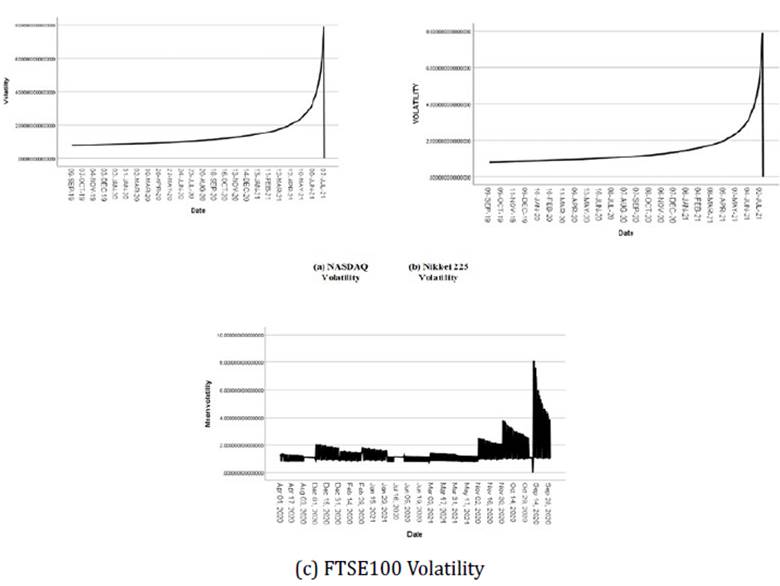
Investors may anticipate 1-2 days per year when the market rises or falls by 4-5% and 1-2 days per year when the market rises or falls by more than 5%. In terms of the DJIA, a 5% change equals around 1,300 points. Compared to Indian markets, the US markets have provided somewhat greater returns with less risk and volatility.
Analysis of the VAR-BEKK-GARCH model
When an occurrence in one nation has a ripple effect on the economy of another, generally more reliant country, this is known as a spillover effect. Downturns in the stock market can have a cascading impact. Subsequently, we examine the stock market's spillover effects as a result of the COVID-19 pandemic.
The estimated model begins with a glance at the graph in Figure 11. The projected volatilities of the returns on the NASDAQ bond index are larger than the squared volatilities of the NASDAQ returns. In general, the stock market is riskier than the bond market, implying that volatility will be higher. Similarly, it can be observed that the three designated periods (using circles) with significantly greater variances correspond to the times marked in Figure 2.
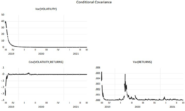
The BEKK-GARCH model for the India-NASDAQ exchange rate is shown in Table 13. According to the variance equation, the probability is less than 0.1. The diagonal matrix with the covariance equation is revealed by the stock market's vo-latility and returns. Because the converted variance coefficients are negative, there is a significant spillover effect across the stock exchange markets.
Table 13 Dynamic BEKK-GARCH model
| Coefficient | Std. Error | z-Statistics | Prob. | |
| C(1) | 1.921064 | 0.006201 | 309.7864 | 0.0000 |
| C(3) | -7.07E-05 | 4.73E-07 | -149.4003 | 0.0000 |
| C(4) | 83.28487 | 49.67990 | 1.676430 | 0.0937 |
| C(6) | 0.995042 | 0.003905 | 254.8141 | 0.0000 |
| Variation Equation Coefficients | ||||
| C(7) | 8.72E-05 | 2.16E-05 | 4.029492 | 0.0001 |
| C(8) | -0.412321 | 0.171445 | -2.404974 | 0.0162 |
| C(9) | 640.4941 | 264.8590 | 2.418245 | 0.0156 |
| C(10) | 1.060679 | 0.118324 | 8.964161 | 0.0000 |
| C(11) | 0.255937 | 0.029843 | 8.576246 | 0.0000 |
| C(12) | -0.153166 | 0.124525 | -1.229998 | 0.2187 |
| C(13) | 0.949384 | 0.011533 | 82.31744 | 0.0000 |
| t-Distribution (Degree of freedom) | ||||
| 11.57170 | 11.57170 | 3.271991 | 3.536591 | 0.0004 |
| Log-likelihood | -2387.285 | Schwarz criterion | 10.65498 | |
| Avg. log-likelihood | -2.623390 | Hannan-Quinn criterion | 10.58912 | |
| Equation: VOLATILITY=C(1)+C(3)*CLOSE(-1) | ||||
| R-squared | -0.091207 | Mean dependent var. | 1.433338 | |
| Adjusted R-squared | -0.093616 | SD dependent var. | 0.952359 | |
| SE of regression | 0.995940 | Sum squared resid. | 449.3293 | |
| Durbin-Watson stat. | 0.003713 | |||
| Equation: VOLATILITY=C(4)+C(6)*CLOSE(-1) | ||||
| R-squared | 0.992533 | Mean dependent var. | 12324.68 | |
| Adjusted R-squared | 0.992516 | SD dependent var. | 1993.482 | |
| SE of regression | 172.4512 | Sum squared resid. | 1347.1957 | |
| Durbin-Watson stat. | 0.003713 | |||
|
Covariance specification: Diagonal BEKK GARCH=M+A1*RESID(-1)* RESID(-1)’*A1+ B1*RESID(-1)*B1 M is an indefinite matrix* A1 is a diagonal matrix B1 is a diagonal matrix | ||||
| Transformed Variance Coefficients | ||||
| Coefficient | Std. Error | z-Statistics | Prob. | |
| M(1,1) | 8.72E-05 | 2.16E-05 | 4.029492 | 0.0001 |
| M(1,2) | -0.412321 | 0.171445 | -2.404974 | 0.0162 |
| M(2,2) | 640.4941 | 264.8590 | 2.418245 | 0.0156 |
| A1(1,1) | 1.060679 | 0.118324 | 8.964161 | 0.0000 |
| A1(2,2) | 0.255937 | 0.029843 | 8.576246 | 0.0000 |
| B1(1,1) | -0.153166 | 0.124525 | -1.229998 | 0.2187 |
| B1(2,2) | 0.949384 | 0.011533 | 82.31744 | 0.0000 |
Source: author's elaboration.
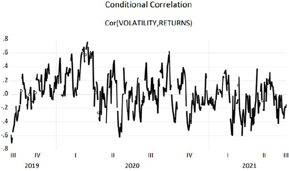
The conditional correlations between the two returns are depicted in Figure 12. The conditional correlation fluctuates over time, as seen by this. For example, the conditional correlation estimate on October 15, 2019, was -0.652, but only 18 days later it had decreased to -2.36. The mean value of the conditional correlation before and after the turning point confirms this. The NASDAQ witnessed a burst in early September 2019 when it rapidly fell (see Figure 12). The NASDAQ's decrease closely corresponds to the year 2020. Before the COVID-19, the correlation was generally negative, and subsequently, it was mostly positive.
CONCLUSIONS
Due to their importance in determining a country's economic situation, financial markets have long been researched from many perspectives. In this context, a re-levant feature of stock markets that has gotten a lot of attention in the economic literature for a long time is the examination of stock returns and volatility. The dispersion of all possible outcomes of an unknown variable is referred to as volatility. It is similar but not identical to risk. While risk is connected to a negative result, volatility, which measures uncertainty, might be associated with a favorable one. Using asymmetric TGARCH models, this article investigated the effects of positive and negative news on volatility in the Indian stock markets during the COVID period of 2019-2021. Given the expiration of the decoupling theory and the consequences of emerging market integration with developed markets, it is necessary to consider the effects of any possible bad news and take precise steps before being trapped in a financial crisis, as was the case with the 2020 pandemic. In this regard, we compared the NASDAQ, Nikkei 225, and FTSE100 stock market indices with the foreign exchange market.
This study aimed to reflect on the effects of volatility spillover from the stock market to the foreign exchange market in a few nations. Data for this study was collected daily from September 8, 2019, to July 9, 2021. The research used the VAR-BEKK-GARCH model to examine asymmetric volatility spillover effects between the stock and foreign currency markets. The findings of this study can help economic policymakers and investors make better decisions regarding international portfolio and currency risk strategies. For NASDAQ, Nikkei 225, and FTSE100, empirical data demonstrate statistically substantial bidirectional volatility spillover between the stock and foreign currency markets. In the case of India, the findings show that stock market volatility spills over into the foreign currency market in a one-way fashion. There is no indication of volatility spillover between the two financial markets in the case of NASDAQ (foreign exchange market and stock market). It was observed that there is an imbalance in volatility spillover across all markets. The research found that the overall persistence of foreign currency market volatility was greater than that of stock market volatility. Therefore, it may harm the country's economic growth. The study argued that stock market volatility has a negative impact on the foreign currency market.
Policy Implications and Future Study
The current study examined the volatility and return of NSE stock indices and NSE sectoral indices before and after the COVID period using SPSS and EViews software simulations. This research also included a comparison of the Indian stock exchange with worldwide markets and a spillover analysis. Fortunately, the worst of the crisis appears to be behind, leaving HR and businesses around the world to figure out what comes next and how work will feel in the future. Organizations rely on market sectors to distribute the most up-to-date information on stock market volatility in their sectors. According to the study, human resource management may solve the issues by implementing equitable and just succession planning to ensure that a firm's reputation is not jeopardized and by implementing incentive schemes at all levels of the organization. These study findings will aid various industries represented by stock market indices that have reacted to the COVID-19 shock, indicating which sectors managed to keep stability and remained resistant to the pandemic. Markets react to a company's growth, cash flow generation, and competitive advantage over time. As a result, the extreme volatility of equities markets offers investors both an opportunity and a risk. The COVID pandemic has impacted stock prices and heightened volatility in Indian stock markets and in the financial sector. Stocks from weakly inter-connected industries can help investors decrease their exposure to protracted uncertainty by including them in their portfolios. Based on statistical analysis, this insight into future directions offers specific sector analysis in the global stock market and determines which country's stock market is the most affected

