Inglés (pdf)
 Articulo en XML
 Referencias del artículo
 Enviar articulo por email
 Citado por SciELO
  Citado por Google
  Similares en
SciELO
Similares en
SciELO  Similares en Google
 Permalink
INTRODUCTION
The economic literature agrees about the positive effect of human capital on labor productivity and, consequently, on wages. In parallel, although subject to less attention, the opposite causality is also observed in the Mexican developing economy, generating a dynamic positive cycle between human capital and wages.
Given that larger wages loose time and budget constraints and increase the incentives for private investment in human capital as well, the positive effect of wages on human capital investment decisions is supported not only by observed data but also by microeconomic theoretical foundations.
Specifically, considering human capital as a function of formal education -that is, letting aside some other sources of human capital formation such as learning by doing-, larger wages: i) provide additional monetary resources to workers, making tuitions and related educational expenses more affordable in societies where guaranteed free access to public education is not normatively or positively implemented; i i) release time and energy resources to workers, making them available for educational purposes -workers receiving lower wages per hour compensate them by working more hours in developing countries, as seen in Mexican statistics (Table 2); and, i i i) considering wages as the returns to human capital, the larger the former, the more incentives for investing in the latter.
By providing a dynamic structural model and its empirical application, it is the aim of this paper to evidence the positive effect of wages on the workers' human capital intertemporal investment decisions, as well as to prove the existence of a virtuous dynamic cycle between wages and human capital. Explicitly, the solution to the model here proposed proves, through its decision rules -policy functions-, the optimality for agents facing higher wages to invest more in education, with the consequent achievement of higher levels of human capital. Whereas model wages remain as positive functions of human capital, closing, this way, the dynamic positive cycle.
The model predicts that there exist two benchmark levels of gross return to human capital and their corresponding wages. Above/below the second benchmark, workers' human capital grows/vanishes in the long run, due to investment being larger/lower than depreciation; at or below the first one, workers stop investing in education.
Whilst the model remains simple, focusing its attention on the optimal intertemporal investment in education when the constraints are loosened due to higher wages, it has two desired characteristics. First, it is able to replicate what is empirically observed in the Mexican economy, in the sense that there exists a virtuous dynamic cycle between wages and human capital, at not very low wages. Second, it has an analytical solution, permitting the achievement of optimal decision rules and the calibration of the parameters using observed data, permitting this way its easy implementation by policymakers and researchers1.
It is worth mentioning that, according to the economic theoretical literature on the formation of human capital, this can be accumulated through different sources, being the principal ones the time devoted to education, whose costs have been modeled as forgone earnings (Ben-Porath, 1967; Brown, 1976), and learning by doing, which can be interpreted as the accumulation of knowledge through working experience (Imai & Keane, 2004). Additionally, some other determinants have been included, such as private education spending (Angelopoulos et al., 2017; Balmaceda, 2021; De La Croix & Michel, 2007); parents' wealth (Balmaceda, 2021); child labor productivity (Fan, 2004); direct costs of schooling (Groot & Oosterbeek, 1992); government expenditure on education (Dissou et al., 2016); and, ability (Huggett et al., 2006).
For parsimonious reasons, or model tractability, all aforementioned determinants have been modeled independently (Brown, 1976; De La Croix & Michel, 2007; Groot & Oosterbeek, 1992), or as a combination of a subset of them, being the former case the methodology followed by this research.
Apropos the previous determinants, we recognize that the opportunity to attend formal educational centers is not guaranteed in the Mexican economy, as has been implicitly assumed. This is due to diverse facts, among others: i) the number of available places in primary, lower, and upper secondary public educational centers is not enough for the demand -a situation which is exacerbated in the tertiary stage, where only a relatively limited number of places are offered; ii) the lack of educational centers in some rural or small urban areas; and, iii) insufficient available time, given that workers with low wages need to compensate their low hourly wage with more working hours, dropping necessarily all or a fraction of schooling hours.
This way, the accumulation of human capital, through formal education, is often conditioned on: i) the capacity of affording private educational expenses, such as tuitions and so forth; ii) the capacity of affording traveling expenses, for attending educational centers in other communities; and, iii) high enough wages, that permit the worker to survive working a fraction of her total available time. As a result, not only the observed nominal and relative number of workers with higher wages that accumulate human capital through formal education is higher than the number of workers with lower wages, but also the amount the former invest in education is higher than that of the latter (see Table 2). This last fact is at the core of our model.
Perhaps, the most controversial difference with respect to previously published theoretical models is that our model predicts the achievement of different levels of human capital, depending on the wage the worker receives, as the analyzed observed data mandates. Thereby, we are implicitly assuming heterogeneous units of labor. In contraposition, preceding models predict convergence to a unique steady-state level of human capital -through different means, such as the inclusion of increasing marginal costs for investing in education- (Ben-Porath, 1967; Brown, 1976), a characteristic that was not possible to support by their empirical application.
On the other hand, our model uses an explicit human capital evolution rule (Angelopoulos et al., 2017; De La Croix & Michel, 2007), which permits qualitative and quantitative theoretical and empirical conclusions; in contrast to implicit human capital evolution rules (Huggett et al., 2006), which limit the theoretical conclusions to be qualitative.
It should be acknowledged that as a result of the flexibility for including variables in econometric regressions, and without the burn of solving a mathematical model, the empirical literature has explored a larger set of human capital determinants. Among them, the introduction of a minimum wage (Cahuc & Michel, 1996; Cubitt & Hargreaves Heap, 1999; Perova & Sarrabayrouse, 2015); taxes (Trostel, 1993); borrowing constraints (Buiter & Kletzer, 1993; De Gregorio, 1996); the innovation rate (Adams & Univer, 1980; Nelson & Phelps, 1966); per capita economic growth (Oketch, 2006); social trust (Yamamura, 2011); federalism and fiscal decentralization (Wolf & Zohlnhöfer, 2009); and, firms' investment in education (Acemoglu & Pischke, 1999).
Finally, certain ideas exploited by this research are not completely new in the literature. Regarding the virtuous cycle, Doner & Schneider (2019) point out that technical and vocational education is simultaneously an "input into production" and a "coproduced good requiring input from both providers and consumers". While the idea of a benchmark wage, above/below which human capital grows/vanishes over time, is in line with the idea of a middle-income trap, followed by these and other authors, and with the segmentation theory, which argues that "vulnerable groups of workers may become trapped in the lower segment of the labour market thereby limiting severely the mobility of employees between the lower and the upper segment" (Leontaridi, 1998).
This paper proceeds as follows: the next section presents the model; then the article puts forth the empirical application of the model to the Mexican economy and discusses some economic policy implications; a later section addresses the conclusions; and, lastly, the details for solving the model and calibrating its parameters are provided in the Appendix.
THE MODEL
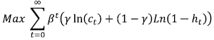
The model here proposed was constructed for modeling workers that enter the job market with a certain amount of human capital. It has one representative agent who seeks to maximize her utility for an infinite period. The agent receives utility from consumption (c) and leisure (lt), being the marginal utility positive and decreasing in both of the utility arguments.
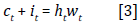
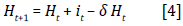
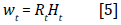
The only source of income of our representative agent is procured by working, being this labor income positively related to the number of working hours (h) and the hourly wage (w); being the last one -in line with Ben-Porath (1967) and Brown (1976) - a function of the gross return of human capital (R t )2 and the level of human capital (H t ), specifically w t = R t H t . The agent is endowed with one unit of time per period, and there exists a human capital evolution rule, which determines that this asset can be increased by investing in education (l t ) and depreciates at a δ rate. Thus, the model assumes the only source of human capital is formal schooling.
The model has a justified assumption, that permits its simplification and an analytical solution. It assumes that the required effort and disutility for working or studying are the same; therefore, considering that in this model the only source of the agent's income is labor income, the resources allocated to acquire one unit of education are the same, regardless if the agent pays it with money -the transition instrument of resources- or time. In this last case, one hour of education is paid with the opportunity cost of it, that is, the hourly wage3.
Basically, our representative consumer needs to decide how to optimally allocate across time her two resources: time and income. By working less, her current leisure increases and consequently her current utility; however, the opportunity cost of decreasing the number of working hours is a smaller labor income, and consequently less available resources for current consumption and investment in human capital, decreasing this way not only current but also future consumption.
Regarding the income resources, they can be allocated either to current consumption or to investment in human capital through a larger expenditure on education; allowing, with the last option, to increase her future labor income. In other words, a larger current expenditure on education means the transfer of resources to the future, which will evolve depending on the marginal productivity of human capital (hR) and the depreciation rate (δ); once those resources are converted in the future into consumption, they modify, depending on the discounted factor (β), the present value of the agent's life utility.
The agent is assumed to belong to a competitive market. As a price taker, she does not have any control over the gross return of human capital4; additionally, she is not expecting the last one to change across time [E"(R ) = E(R t+1 ) = R]. Consequently, the agent knows that the only path for positively affecting her wage is by investing in human capital, becoming the former an endogenous variable. Finally, we have to say that, as in Brown (1976), human capital is disembodied, meaning that its return is independent of the number of working hours chosen by the agent.
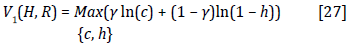
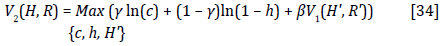
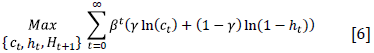
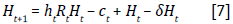
Formally, our representative agent maximizes the present value of the sum of her current and future utility
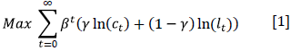
Subject to a time constraint
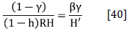
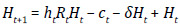
A budget constraint
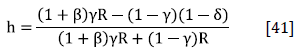
A human capital evolution rule
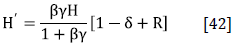
And the agent's wage function
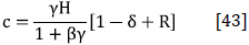
Solution of the Model
The model is solved through dynamic programming and sequential methods. As it is known, the first technique allows to determine the decision rules for each agent's choice variables (c t , i t , h t , l t , H t+1 ). Thus, the optimal allocation of resources to each of these variables can be determined at any period, depending only on the value of the state variables (H t , R t , w t ) and the parameters; where H t and w t are the endogenous state variables and R t the exogenous state one.
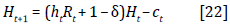
For solving the model using dynamic programming we simplify the notation by substituting H t+1 , H t , R t , w t , c t and h t by H', H, R, w, c and h, respectively. Additionally, using the time constraint, l t is substituted by 1 - h t in the utility function; while the budget constraint and the agent's wage function are merged with the human capital evolution rule, obtaining the following problem to be solved
Subject to
Using the Bellman equation
Subject to
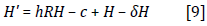
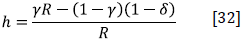
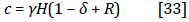
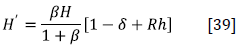
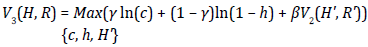
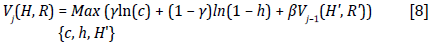
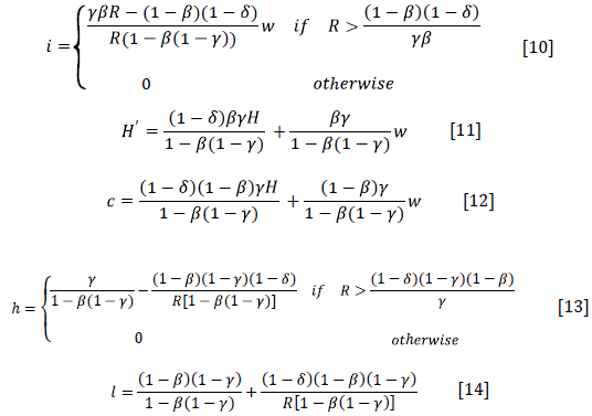
it is possible to obtain the following decision rules for i, H', c, h and l, which only depend on state variables and parameters. For more details regarding the calculation of the decision rules see the Appendix.
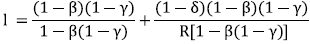
As can be observed in the previous decision rules, the optimal futu re level of human capital is a positive function of the hourly wage; that is,
 . Concurrently, given that Equation [5] is true at every period, the hourly wage is a positive function of human capital; that is,
. These facts mathematically prove the existence of a virtuous dynamic cycle between wages and human capital.
. Concurrently, given that Equation [5] is true at every period, the hourly wage is a positive function of human capital; that is,
. These facts mathematically prove the existence of a virtuous dynamic cycle between wages and human capital.
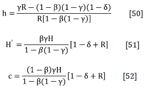
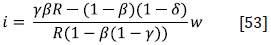
It is worth to notice that according to Equation [10], the agent will decide to invest in education as long as the gross return of human capital (R) is larger than
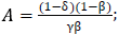 being that this level of R corresponds to the first benchmark gross return and its corresponding wage, at and below which the agent stops investing in education. By the same token, in accordance with Equation [13], the agent will offer a positive number of working hours only if R is above
 . While according to Equations [11] and [12], the minimum level of human capital for the next period (H] and consumption (c), when the wage is equal to zero, are
 and
and
 , respectively.
Using the decision rules, the predicted values of the choice variables -at different gross returns of human capital and wages- are depicted in Figure 1.
Intertemporal Optimal Conditions and Calibration of Parameters
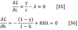
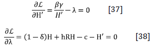
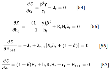
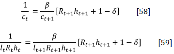
The model permits the achievement of the intertemporal optimal conditions, given by the Euler equations, as well as the calibration of its parameters, by defining these last ones as functions of observable variables. See the Appendix for further details.
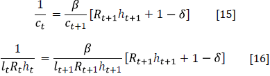
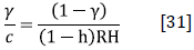
As usual, the optimal allocation of resources across time requires the marginal utility of consumption at any period t (Equation [15]) to be equal to the discounted marginal utility of consumption at period t + 1, multiplied by the marginal productivity of human capital plus one minus the depreciation rate. An analogous interpretation should be provided to the marginal utility of leisure (Equation [16]).
Finally, through the first-order conditions of sequential methods, the policy function for c, the human capital evolution rule, and the Euler equation, the parameters are calibrated.
Benchmark Human Capital Gross Returns and Their Corresponding Wages
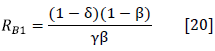
The Section "Solution of the Model" presented the first benchmark human capital gross return, at and below which the agent stops investing in education
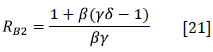
The proposed model permits to determine a second benchmark human capital gross return, and its corresponding wage for each level of human capital, at which workers invest in their education the required amount for maintaining their initial level of human capital over time.
A virtuous cycle is generated above this second benchmark wage, because by investing in education more than the required amount for compensating its depreciation the worker's human capital grows, and therefore also her wage; given that the latter is a function of the former.
In order to find the second benchmark human capital gross return, we substituted Equation [5] in [11], solved for R, defined H' = H, and simplified the solution
R B1 and R B2 are quite useful for finding the benchmark wages -see Section "The Benchmark Mexican Human Capital Returns and Wages" and the formulas used in Table 2-. The reader must be aware that neither our gross nor our net human capital return refers to the return on education. Our gross human capital return is the return to labor, conditional on the agent's level of education, when she exploits her capital as much as possible, that is, when her leisure is zero (R = total labor income / human capital x fraction of available time working). Thus, this figure is bigger than our net human capital return (R N = total labor income / human capital). And both of them are larger than the narrower returns to education, experience, etcetera, found in the economic literature about the Mexican labor market (Harberger & Guillermo-Peón, 2012; Morales-Ramos, 2011; Ordaz-Díaz, 2008) by using the Mincer (1974) equation.
The Temporal Path of Investment, Human Capital, and Consumption at Different Gross Human Capital Returns
To predict the temporal path of investment in human capital, human capital stock, and consumption, at different gross human capital returns, a difference equation is defined. It is constructed by merging the budget constraint (Equation [3]) and the human capital evolution rule (Equation [4])
rearranging the previous equation, we get
To solve the previous first order difference equation the following lemma is used.
Lemma 1 The curve
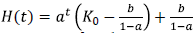 is the solution to the first order difference equation H
t
= αH
t-1
+ b; where α ≠ 1, a and b are constants, and K
o
= H(0).
is the solution to the first order difference equation H
t
= αH
t-1
+ b; where α ≠ 1, a and b are constants, and K
o
= H(0).
By substituting Equation [5] in [12], substituting the resulting equation and Equation [13] in Equation [22], and according to the previous lemma, the curve
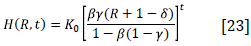
is the solution to the first order difference Equation [22]. In different words, Equation [23] returns the values of human capital over time, depending on the values assigned to R and the parameters.
By substituting Equations [5] and [23] in [12], we get the temporal path of consumption [c(R, t)] as a function of the exogenous state variable (R), time, and the parameters
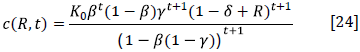
Lastly, by substituting Equations [5] and [23] in Equation [10] we get the temporal path of investment [i(R, t)]; which also only depends on parameters, the state variable R, and time
Once the parameters are calibrated for a given economy, the previous three equations allow plotting the model-predicted temporal paths of investment, human capital, and consumption, at different gross human capital returns. This is done for the Mexican economy in section "Model Simulation" .
EMPIRICAL APPLICATION AND ECONOMIC POLICY IMPLICATIONS
The empirical application of the proposed model is provided in this section; applied to the Mexican developing economy, although it can be applied to any economy. More specifically, using the model it is presented: i) the Mexican dataset and its descriptive statistics; ii) the calibration of the parameters; iii) the comparison of the model predicted human capital temporal path versus the Mexican observed data; iv) the benchmark human capital gross returns and corresponding wages, above which there exists a virtuous dynamic cycle; v) the simulation of the variable values over time; and, vi) the discussion of some economic policy implications.
Datasets and Descriptive Statistics
The datasets used in this research correspond to the National Surveys of Household Income and Expenditure (ENIGHs; INEGI, 2014, 2016, 2018). ENIGHs5 are surveys conducted every two years by the Mexican National Institute of Statistics and Geography (INEGI). With these datasets, we constructed a pseudo-panel that provides the observed values of the variables involved in the model.
ENIGHs 2014, 2016, and 2018 surveyed a total of 19,479, 70,311 and 74,647 households, respectively, with information for each household member. This way, we have information for 73,592, 257,805 and 269,206 surveyed persons, respectively. Once each household and members are multiplied by its respective expansion factor, the surveys become representative of the entire Mexican population. The current research uses the final figures, shown in Tables 1 and 2.
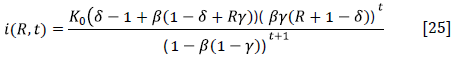
As we can observe in Table 1, according to ENIGH, during 2018 there were a total of 47 million workers in the Mexican economy, of which 45.2 million were remunerated and 1.8 million non-remunerated. Of the remunerated workers, 12.9 million received non-labor income in addition to their labor income; while, in accordance with our model, the income of 32.3 million workers relied only on labor.
Concerning the schooling characteristics, we can observe that out of 36.5 million people that attended school during 2018 in Mexico, 4 million were workers; while out of 18.9 million people that spent on education, 2.2 million were workers.
Table 1 Descriptive Mexican Population Statistics by Labor and Schooling Conditions
Source: Own elaboration using ENIGHs 2014, 2016, and 2018.
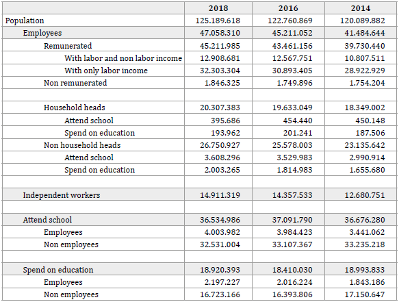
Given that we are interested in isolating the effects of wages on own private investment in education, we need to exclude from our sample all those individuals that receive resources by means other than their own labor. With this target in mind, considering that at the interior of Mexican households it is a common practice that household heads support the education of non-household heads -among them working children and teenagers-, this empirical research was done considering only household heads whose income comes only from labor -avoiding, this way, intra-household educational transfers-. Their labor and investment in education characteristics, by quintiles of hourly wages, are exposed in Table 2. As can be observed, as of 2018 there existed a total of 13.6 million workers, without non-labor income, that were household heads.
Several relationships between variables are worth to be noticed in Table 2. The hourly wage, as well as the labor income per worker, is an increasing convex function of the number of schooling years; in other words, the marginal returns to education are positive and increasing. The number of weekly working hours is negatively correlated with the hourly wage. The number of workers that invest in human capital through spending on education, as well as the amount these workers spend on it, is positively correlated with the hourly wage; while the average amount spent on education, considering all workers, is an increasing convex function of the hourly wage.
Table 2 Workers (Household Heads Without Non-Labor Income) by Labor and Investment in Education Characteristics1 (in Mexican pesos, October of 2018 prices)
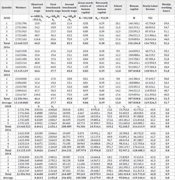
Source: Own elaboration using ENIGHs 2014, 2016, and 2018. The interested reader may convert the figures to USD, using the following exchange rates for 2014, 2016, and 2018, respectively: 13.366492, 19.217797, and 19.360464 Mexican pesos per one USD, which correspond to the average dairy exchange rate during the period ENIGH surveys were done: 21th August to 28th November for 2016 and 2018 ENIGHs, and 11th August to 28th November for 2014 ENIGH.
1/ Statistics of employees that are household heads and which only source of income is labor. All statistics -except for workers, workers attend school and workers invest in education- correspond to the average by quintile or total average.
2/ Average own monthly educational expenditure per worker, considering only those workers that invest in education.
3/ Average own monthly educational expenditure per worker, considering all workers of the same quintile.
4/ Average consumption per worker, considering only those workers that invest in education.
5/ Average consumption per worker, considering all workers of the same quintile.
6/ Where male = 1 and female = 0. Thus, if the value in the table is 0.8 means 80% of the sample is male.
Calibration of Parameters
In order to recover the values of the model's parameters it is possible to estimate or calibrate them. Both techniques have their supporters and critics; for example, according to Cunha et al. (2021), the estimation of human capital parameters has certain issues such as "anchoring" measurement error" and the correlation between observed inputs and unobserved error terms that affect estimates of the parameters of human capital production functions". The calibration technique is followed in this research.
In this case, the calibration procedure6 requires evaluating the average investment workers -in our case household head Mexican employees- necessitate for achieving the amount of human capital (H) they possess; for doing this we multiply the average required expenditure for getting one year of education during the whole analyzed period" that is $23,679.9, times their average number of schooling years. Thus, in the case of 2014, 2016, and the total average, H = $23,679.9 x 13.0 = $307,838.8.
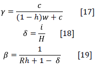
Following Equation [18], for calibrating ô, the average yearly investment in human capital is divided by the average amount of human capital -expressed in Mexican pesos- of Mexican workers. Therefore δ = i/H = 23,679.9 / 307,838.8 = 0.0769.
For calibrating β, using Equation [19], one is divided by Rh + 1 - δ. Therefore β = 1 / (0.8418*0.4613 + 1 - 0.0769) = 0.7626.
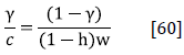
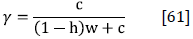
For calibrating у we assume there are 16 available daily hours for distributing among leisure and working; this way, economic agents have 112 weekly available hours. According to the data presented in Table 2, Mexican workers decide to spend on average 51.6608 weekly hours working and consequently 60.3392 weekly hours on leisure, therefore l = 0.5387. Following Equation [17], being aware that Iw is the monetary value of leisure time, w = RH, and using annual data -same results as with hourly data- we obtain γ = $95,846.6 / (0.5387 * 0.8418 * $307,838.8 + $95,846.6) = 0.4071.
It is worth noticing that the only parameter that can be affected by changing the total number of available weekly hours is γ. That is, δ and β do not change by assuming the agent has fewer or more available hours per week. 112 weekly available hours were chosen, assuming the agent needs to sleep 8 hours per day.
These results can be compared with those of the economic literature. Concerning the depreciation rate, our results are in line with those of Vignoli (2012), which were between 0.0342 and 0.0793, and those of Castillo-Aroca (2016), which were between 0.0549 and 0.1677. On the other hand, Campbell & Hercowitz (2009), as well as Eden & Gaggl (2017), obtained estimations of у between 0.35 and 0.63. Finally, although Issler & Piqueira (2000) estimated the values of the discount factor β between 0.64 and 0.99, our calibrated value for ß is below the usual value encountered in the literature. This is because the standard formula for calibrating it, β = 1 / (Rh + 1 - δ), comes from the Euler equation, where Rh represents the marginal productivity of the input factor, equal to its return in a competitive market. Given that this is located in the denominator and that the return is higher for human than for physical capital, it is clear the value for ß must be lower when the human instead of the physical capital is analyzed; being the last case the usual one.
Comparison of the Model Predicted Human Capital Temporal Path Versus Mexican Observed Data
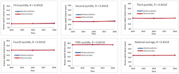
By substituting the calibrated parameters in the policy function that determines the optimal agent's decision regarding the next period human capital (Equation [11]), the model-predicted human capital temporal path is obtained, and then compared with the observed data in Figures 2 and 3. The only difference between these two Figures is that Figure 2 uses the observed average gross yearly return of human capital per quintile, from 2014 to 2018, while Figure 3 uses the observed national average of the same variable -both of them located in the sixth column on Table 2.
It is necessary to be aware that a Mexican public panel data survey that interviews the same sample of people in the long run, permitting to follow their live history -as NLSY or PSID datasets for the American society-, does not exist7. Consequently, for the Mexican case, it is not possible to meticulously compare the model-predicted values with the decisions of the same people across time. However, it is possible to perform the comparison of the model-predicted values with an observed representative group of people that shares similar characteristics, that is, a pseudo panel.
As can be observed, the model predictions fit the data in 10 of the following 12 cases. The exceptions are the first and fifth quintiles, when the observed gross return by quintile is used. These exceptions are very helpful for understanding the limitations of the model and the used dataset.
In the first quintile, the observed hourly wage is below the first benchmark hourly wage -see Table 2-, so, according to the model, the agent stops investing in education. This forecast is well supported by the observed data, considering the number of workers that invest in education and the amount they invest. Therefore, the plot is showing how human capital depreciates when investment is zero. For improving the fit of the first quintile, it would be necessary to apply the depreciation to the observed data.
In the fifth quintile, the gross return is quite high -1.38-, so workers usually increase their rate of consumption and invest a fraction of their high income in physical assets. But this model uses a linearized Cobb Douglass utility function, which is characterized for holding constant the fraction of income addressed to consume or invest when prices or income change. Additionally, the model does not consider the existence of other physical assets for investing; so, with such a great return, all additional income, multiplied by its corresponding investment fraction, will be allocated to human capital. The model can be complicated to include these other facts, but then it will lose parsimony and an analytical solution.
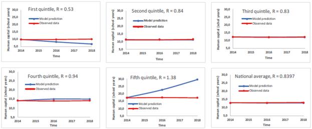
Figure 2 Human Capital Temporal Path by Quintile, Observed vs Model Prediction, With Average Quintile Observed Gross Returns -R-
The Benchmark Mexican Human Capital Returns and Wages
To find the benchmark Mexican human capital gross returns, it's only required to substitute the calibrated parameters in Equations [20] and [21], obtaining R B1 = 0.7062 and RB2 = 0.84178. To obtain the corresponding benchmark hourly wages per level of human capital, it is necessary to convert all variables into the same units of measure -in this case, Mexican pesos- and realize that given Equations [2], [3], and [5] are true at any time, then R, R B1 , and R B2 are gross rates of return of human capital, that is, assuming the human capital is used all the available time. So, the benchmark hourly wages are obtained by multiplying the values of R B1 and R B2 times the amount of human capital -in Mexican pesos- times the fraction of time that the human capital is used -the fraction of time the worker works- and dividing the result by the number of hours the employee works during the year. The results are shown in Table 2, in the columns first and second benchmark hourly wage.
Model Simulation
By substituting the calibrated parameters, β = 0.7626, δ = 0.0769, and γ = 0.4071, in Equations [23], [24], and [25], which were defined for forecasting the variable values using the model, we obtain the temporal paths of human capital [H(R, t)], consumption [c(R, t)], and investment in human capital [i(R, t)],as a function of any gross human capital return and time
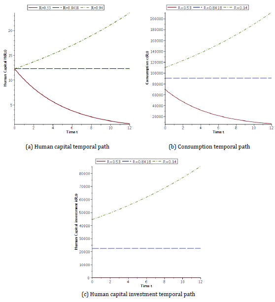
Figure 4 Model Simulation of the Temporal Path of Relevant Variables, at the Gross Return (R) of the First Quintile, Second Benchmark, and Fourth Quintile
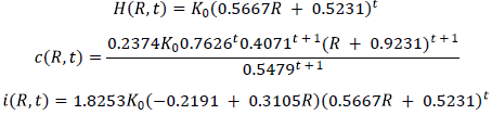
Figure 4 displays the eimulati6n of the 3 previous variables, for 12 periods, at three different human capital returns: R 1 = 0.53, which is the observed average human capital gross yearly return of the first quintile; R 2 = 0.8418, which corresponds to the second benchmark wage, estimated with Equation [21]; and, R 3 = 0.94, which is the observed average human capital gross yearly return of the fourth quintile (see Table 2).
Economic Discussion and Policy Implications
It is possible to observe, in Table 2, that the number of workers that attend school is a positive function of the hourly wage; being this figure, by wage quintile, 321.9% higher for the fifth quintile (84,465 workers) than for the first one (20,018 workers). This relationship holds even if you consider only those workers that attend public schools; in other words, if you consider those workers that pay for their education only with the opportunity cost of their time. In this last case, the number of workers increases, from the first to the fifth quintile, from 13,467 (20,018 workers that attend school minus 6,551 that invest in education) to 38,692.
Thus, the virtuous cycle between wages and human capital holds, even if you consider only those workers that do not pay directly for their education but instead pay it indirectly with the opportunity cost of their time. This can be explained by realizing that workers earning lower wages have fewer resources (time) for allocating to education, given that they have to work more hours to compensate their lower wages; workers of the first quintile work 59.6 hours per week, while workers of the fifth quintile work 44.0 hours per week.
From the analysis in the previous sections stems diverse economic policy implications. As it is possible to observe, in Table 2, during 2018 Mexican workers in the fifth quintile had 72.3% more years of education than workers in the first quintile.
Nevertheless, their hourly wage was 8.37 times bigger, that is, 737% larger. This disproportional increment in their hourly wage was primarily due to the market bought them 384.7% more expensive each unit of human capital, in other words, each school year -from $1.38 to $6.69 per hour per school year.
There are different related theoretical ways for explaining the previous fact: i) There exists one labor market, with homogeneous units of labor, where human capital has positive increasing marginal returns; ii) the wage inequality is based on the heterogeneous nature of workers, being the different investment in human capital the primary cause of this inequality (Mincer, 1974); putting it differently, the more educated worker may earn a higher wage because her higher education is translated into higher marginal productivity; iii) heterogeneous units of labor, in this case units of human capital, traded in several labor markets, are traded as a unit. Therefore, one worker with 16 years of education is not interchangeable with 4 workers, each with 4 years of education, because their quality of labor and productivity are different; and, iv) accepting the arguments of the segmented labor market theory, that is, moving away from the neo-classical theory, "the labour market is not a single competitive market, but is composed of a variety of non-competing segments between which rewards to human capital differ because institutional barriers prohibit all parts of the population from benefiting equally from education and training" (Leontaridi, 1998).
Moving from the first to any other option means transiting from general increasing marginal returns to constant returns for each level of human capital; something that was exploited by the proposed mathematical model.
In any case, we can derive the following policy implication. If the market buys on average each unit of human capital at a price 384.7% higher when it is sold by a worker with 17.4 years of education than when it is sold by a worker with 10.1 years of education, it's because the increment in productivity must be similar. So, once again in the economic literature, if the problem of a given society is low productivity, the straightforward path for solving it is by increasing education.
As will be discussed in the following section, the observed wages of around 40% of Mexican workers are below their second benchmark wage; that is, their human capital coming from formal education decreases over time. This fact has diverse consequences if we relate it with the conclusions of the economic growth literature, given that low wages decrease the level of human capital of workers, and therefore their productivity and the economic growth rate of the country. Thus, the Mexican government economic policy of decreasing wages, for different targets, seems even less plausible.
With the idea of decreasing production costs and consequently increasing the competitiveness of the country, promoting this way the attraction of international enterprises to the country, as well as reducing the unemployment rate, the real Mexican minimum wage has been decreased to around one-third of its value during the last 45 years, being nowadays one of the lowest ones in Latin America. According to the conclusions of this research, more widely developed in the next section, this policy limited the human capital accumulation -and therefore the productivity- of those workers that earn one minimum wage, given that it is located below the second benchmark wage.
CONCLUSIONS
Grounded in the theoretical and empirical results exposed in the current paper, two main conclusions can be derived from this research, mathematically proven and empirically suggested. There exist both: i) a positive effect of wages on human capital investment; and ii) a virtuous dynamic cycle between wages and human capital.
Theoretically speaking, these conclusions are mathematically proved through a dynamic structural model, where wages are treated, following the economic literature, as a positive function of workers' human capital. On the other hand, the solution to the model demonstrates that the optimal intertemporal investment of workers in their own human capital, provided by a decision rule, is a positive function of their wages, closing this way the virtuous dynamic cycle.
These theoretical results were tested against observed data, using official statistics from a developing Mexican economy. After calibrating the parameters and performing the model simulation, it was possible to observe that the model prediction, regarding human capital level, behaves in standard cases as observed data.
Empirically speaking, the constructed and presented statistics (Table 2) support the consistency of the theoretical conclusions and speak by themselves. The hourly wage, as well as the labor income per worker, is an increasing convex function of the number of schooling years; in other words, there exist positive and increasing marginal returns to education. Also, the number of workers that invest in human capital through spending on education, as well as the amount these workers spend on it, is positively correlated with the hourly wage; in the same line, the average amount spent on education, considering all workers, is an increasing convex function of the hourly wage.
The proposed model is able to calculate two benchmark human capital gross returns -Equations [20] and [21]- and their corresponding hourly wages per level of education. At or below the first benchmark hourly wages (fourth column in Table 2), workers stop investing in education; below the second benchmark hourly wages (fifth column in Table 2), workers' investment in human capital is not enough to offset its depreciation, provoking their human capital to vanish in the long run. Intuitively speaking, below the second benchmark hourly wage for each level of human capital, workers do not find it profitable to continue investing in their human capital after entering the job market, or their budget constraints do not allow them to continue doing it; so, they let their human capital, coming from formal education, lessen in the long run.
For the Mexican society, as of October 2018, the observed hourly wages per quintile were $13.9, $24.2, $33.3, $48.7, and $116.4 Mexican pesos for workers with 10.1, 11.5, 12.3, 14.2, and 17.4 school years, respectively. While the corresponding second benchmark hourly wages were $21.4, $23.7, $33.0, $43.3, and $75.9. Thus, all workers of the first quintile are located below the benchmark wage and the average wages of the second and third quintiles are almost the same as their corresponding benchmark wage, so around half of them are below the benchmark wage. Summing up, unfortunately, around 40% of Mexican workers have a wage that locates them below their second benchmark wage (see Table 2); consequently, their human capital, coming from formal education, will decrease over time.
Thus, if the target is a larger accumulation of workers' human capital, the conclusions suggest the need to increase the wages of around 40% of the workers located on the lowest side of the wage distribution and setting them above their corresponding second benchmark wage. This can be done through different sources, such as regulations and incentives. Additionally, regarding the whole wage distribution, the policy-maker must be aware that the higher the wages the stronger the effect of the virtuous dynamic cycle. These results are especially important for developing societies, where low wages, a large wage distribution, and a relatively international low level of human capital are representatives, as in the Mexican case.
Some limitations must be acknowledged, as well as the necessity of future research on the topic. One of the strengths of the mathematical model here presented consists in that it has an analytical solution, which means the solution provides, in addition to a theoretical framework, a set of equations where the user only needs to plug the observed variables, provided by a dataset, and the equations will return the value of the parameters (Equations [17], [18], and [19]), the optimal decisions of the economic agent (policy rules, Equations [10] to [14]), and the forecast path of the variables (Equations [23], [24], and [25]).
Thus, this paper provides a mathematical theoretical framework which policymakers and researchers may easily use to support their empirical research, without the necessity of proposing and solving a dynamic theoretical model using numerical methods. However, the opportunity cost of having an analytical solution is not complicating the model too much, sacrificing other relevant variables or including them indirectly, in this case ability and time, respectively, for explaining the accumulation of human capital. In the same line, the model does not include workers' physical assets, that permit the agent to have non-human capital alternatives where to invest her optimal resources transferred to the future. As a result, at very high wages, the model forecasts the accumulation of human capital increases over time more than what is observed.
Concerning the empirical application, given that no Mexican public panel data survey that follows the live history of people exists, it is not possible to accurately compare the predicted values with the decisions of the same people across time. Thus, future applications of the proposed model in other developing societies, where access to education may not be normatively or positively enforced, and that have panel data surveys, would be enlightening.
Finally, the indirect and direct positive effects of increasing wages on the economy are broad. This research covered only its direct effect on human capital accumulation; however, the increment of wages has other positive effects on: i) economic growth, through human capital accumulation and therefore productivity; ii) the purchasing power of workers and therefore in consumption and aggregate demand; iii) investment in physical capital, given the price of the other production factor (labor) increases; and, iv) reduction of violence, due the increase in the opportunity cost of committing crime.
Thus, there are several channels through which increasing wages contribute to economic targets, especially in developing societies, where wages are characterized for being very low. A lot of research on these topics is still necessary, by using diverse datasets, variables, econometric and mathematical techniques. The opportunity for doing relevant research in the area is broad and the invitation is open.