


 English (pdf)
 Article in xml format
 Article references
 Send this article by e-mail
 Cited by SciELO
  Cited by Google
  Similars in
SciELO
Similars in
SciELO  Similars in Google
 Permalink
Atmospheric aerosols are of global importance because they affect the climate via direct and indirect radiative forcing and adversely impact the human health and ecosystems (Dahari, Latif, Muda & Hussein, 2020). Air pollution continues to be a growing problem for human health in terms of short and long-term effects and is a burden on public health systems around the world (Maesano et al., 2020; Yang et al., 2020). One of the main pollutants that contributes to the deterioration of air quality is particulate matter (PM). The increase in the urban PM is mainly associated with the concentration of industrial activities and the increase in the number of motor vehicles (Terrouche et al., 2016; Zafra-Mejía, Gutiérrez-Malaxechebarria & Hernández-Peña, 2019). Because of this, many Latin American countries have decided to strengthen the active monitoring of air pollution in urban areas in order to control atmospheric pollutants (Palacio, Zafra & Rodriguez, 2014; Franck, Leitte & Suppan, 2014). The impacts of PM on human health are associated with a reduction in cardiopulmonary functions and with an increase in mortality from cardiovascular disease, the occurrence of asthma in children, and the risk of cancer (Hou, An, Tao & Sun, 2016; Maesano et al., 2020).
Dockery et al. (1993) reported that diseases such as bronchitis and chronic asthma were positively correlated with PM concentrations. In a European study conducted in 15 western European cities on air pollution and its effects on public health, it was reported that an increase of 50 Mg/m3 in PM10 concentrations could cause a 2.1% increase in the human mortality rate (Katsouyanni et al., 1996). Another study conducted with the support of the United States Environmental Protection Agency (US EPA) on the effects of air pollution on the respiratory health of people in Chinese mega-cities (Guangzhou, Wuhan, and Chongqing), it was observed that the PM10 concentration was directly related to the rate of childhood lung dysfunction (Liu, Xu & Yang, 2018). Lacasaña et al. (1999) and Hernández et al. (2013) reported that the effects on human health from extreme events of air pollution were short-term. This study reported latency periods of up to seven days.
Studies reported that the AC plays an important role in the transportation and dispersion of PM10, and is significantly related to temperature variation at altitude (thermal gradient) and wind speed (Srinivas, Venkatesan, Somayaji & Indira, 2009), with this last variable also depending on land surface characteristics (Chambers et al., 2015; Zafra, Ángel & Torres, 2017). Related to this, Lee, Ho, Lee, Choi and Song, (2013) reported that in Seoul (Korea), under extreme atmospheric stability conditions (thermal inversion) the PMl0 concentrations tended to increase significantly (PM10 > 100 Mg/m3). Vecchi, Marcazzan and Valli, (2007) reported a 13% increase in PM10 concentrations in Milan (Italy) under prevailing conditions of nighttime atmospheric stability (low dispersion), despite a reduction in the emission sources (traffic, domestic heating, and industries). This study also reported that, under conditions of daytime atmospheric instability (high dispersion), the PM10 concentrations tended to decrease.
As can be seen, it is relevant that urban public health control agencies study the possible relationship between PM concentrations and the atmospheric condition (AC) that prevails in a given area. In this way, it is also relevant to study the possible relationship between AC and the human mortality rate associated with PM concentrations.
This study was conducted in the city of Bogotá, Colombia, a high-altitude Latin American mega-city with a population of 8.85 million inhabitants in 2015. It is located in a large inter-mountain valley in the eastern Andes (04o36'35"N-74°04'54"W) at an average altitude of 2600 masl. Its tropical mountain climate is characterized by large temperature variations per hour (maximum variation = 12 °C). The city is recognized as the urban centre with the highest population density (26,000 inhabitants/km2) and the third-highest air pollution level in Latin America (Sarmiento, Hernández, Medina, Rodríguez, & Reyes, 2015). According to Montoya, Cepeda and Eslava, (2004), atmospheric instability conditions during the day are recorded in the city due to the increase of solar radiation until noon and afternoon. During the night, the wind speed is very low, which produces stable and neutral atmospheric conditions. Therefore, due to the interaction between the degree of pollution and the particular climatic characteristics of the city, the development of this study is of interest when it comes to understanding the behaviour of PM10 and the associated mortality rate according to atmospheric conditions.
This article aims to study the relationship between AC and the human mortality rate associated with PM10 concentrations in this high-altitude megacity of Bogotá (Colombia). The study was developed from the available PM10 information per hour between the years 2007-2012 from three automatic monitoring stations located throughout the city. This study hopes to increase knowledge about: (1 the behaviour of PM10 contamination in high-altitude megacities in developing countries; (2) the possible relationship between AC and the daily mortality rate associated with PM10 in megacities.
Materials and methods
Data collection
The three automatic monitoring stations were located in Kennedy (S1), Barrios Unidos (S2) and Guaymaral (S3) in Bogotá, Colombia. These stations were selected because they showed the maximum (S1) and minimum (S2 and S3) concentrations of PM10 during the study period. Additionally, the selected stations did not have any significant changes in land surface coverage, but they had information about climatic variables allowing for a determination of the AC. The tropical mountain climate showed an average daily temperature of between 13.3 -14.3°C and wide temperature variations per hour with variations between 7.2 - 19°C. Table 1 shows the main characteristics of each monitoring station. The locations of the monitoring stations are shown in Figure 1.
Table 1 Characteristics of the location zones of each monitoring station
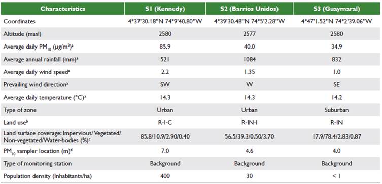
Note: a During the study period; b R = Residential, I = Industrial, C = Commercial, and IN = Institutional; c Within a l600-m radius with center in the monitoring station; d With respect to the land surface.
PM10 sampling system
The sampling period lasted for six years (01/01/2007-12/31/2012). This time interval was selected because the areas surrounding the monitoring stations showed no significant changes in land surface coverage (impervious, vegetated, non-vegetated, and water-bodies; see Table 1).
Thus, during the sampling period, the possible effects of the variation of land surface coverage in the AC (vertical gradient of temperature and wind speed) at each sampling site was minimized. The hourly PM10 sampling system consisted of continuous-monitoring equipment which used beta ray attenuation (Met One Instruments, BAM 1020). The sampling protocol followed the guidelines set forth by the United States Environmental Protection Agency in EPA/625/R-96/010a-IO-1.2 (U.S. EPA, 1999). The equipment's constant flow rate was 16.7 1/min. The lowest detection limit was 3.6 µg/m3 and 1.0 µg/m3 for hourly and daily sampling intervals, respectively. Resolution in the measurement was 0.24 Mg in a range of 1 mg. The precision was ± 8% for hourly intervals and ± 2% for daily intervals.
Atmospheric condition
For each monitoring station, the AC was determined based on the Pasquill (1961), Turner (1964), and Gifford (1976) methodologies, using hourly data on wind speed and solar radiation. The prevalence of the AC was determined following the methodologies proposed by Zoras, Triantafyllou and Deligiorgi, (2006) and Chambers et al. (2015) according to their hourly frequency. Differences in hourly frequency between monitoring stations were evaluated by applying the Kruskal-Wallis test, which is a non-parametric alternative test to a one-way ANOVA. The CA data distribution was validated with the Shapiro-Wilk test, identifying a non-normal distribution (df = 24; p values <0.001). The CA states were defined on a quantitative scale according to the categories: 1 = stable, 2 = slightly stable, 3 = neutral, 3.5 = neutral to slightly unstable, 4 = slightly unstable, 4.5 = slightly unstable to unstable, 5 = unstable, 5.5 = unstable to very unstable and 6 = very unstable. Finally, a graphical comparison between PM10 concentrations and the AC was presented for each monitoring station.
Air quality standards
The standards selected to assess air quality in the study areas were Colombian Resolution No. 610/2010 (MAVDT, 2010) and air quality guidelines of the World Health Organization (WHO, 2005). These standards established that the maximum permissible levels allowed for PM10 are 100 and 50 Mg/m3 for an exposure time of 24 hours, respectively. The frequency of exceedance of these maximum permissible levels during the entire study period was analysed for daily and monthly time scales.
Following the daily concentrations of PM10 and the reference legislation, quartiles (Q) were established in order to assess the risk to public health. Average daily PM10 concentrations were calculated by month and later organized in order of precedence. The three months that exhibited the highest PM10 concentration (greatest public health risk) were assigned to the first quartile (Q1). The quartiles Q2, Q3 and Q4 were assigned according to PM10 concentration in order of precedence. Thus, the three months with the lowest average PM10 concentration were assigned to the last quartile (Q4), representing the lowest risk group for public health.
The increase in the human mortality rate related to PM10 for the study areas was calculated. This calculation was based on the guidelines established by WHO (WHO, 2005). The results of studies at a global level suggested that the public health risks related to short-term exposures to PM10 were probably similar in cities in developed and developing countries, with an increase in the daily mortality rate around 0.50% for each l0 Mg/m3 increase in PM10 (WHO, 2005). Thus, this study assumed an increase in the daily mortality rate of 0.50%. These increases in the daily mortality rate were calculated from the maximum 24-h limit established by WHO for PM10 (50 Mg/m3).
PM10 data analysis
For all monitoring stations, the hourly variation of PM10 concentration was evaluated for the entire study period (n = 24, per monitoring station). The daily variation of PM10 concentrations was evaluated using a 24-hour moving average. The non-normal distribution of PM10 data was determined with the Shapiro-Wilk test (p-values < 0.048). Spearman's correlation coefficient (rs) analysis was carried out to assess the relationship between monitoring stations according to the hourly and daily PM10 concentration. Additionally, to assess the hourly variation of PM10 concentrations at each monitoring station, a standard deviation was used. All statistical analyses were carried out using IBM-SPSS V.19® software.
A graphical comparison between the hourly variation of average PM10 concentration and average AC was carried out to study the influence of the hourly cycles of PM10 emissions from motor vehicles and industries located across the entire study area. Finally, the hourly and daily PM10 concentrations of monitoring stations located in areas with predominantly impervious land surface coverage (S1) were compared with the concentrations of stations located in areas with predominately vegetated land surface coverage (S2 and S3). The previous analysis also considered the prevailing AC with relation to the type of land surface coverage (LSC). In this study, four types of urban LSC were considered: vegetated (trees and grasslands), non-vegetated (bare soil), impervious (roof tops, pavements, and footpaths), and water bodies (rivers, lakes, and wetlands). In the selected monitoring stations, there was no LSC variation during the PM10 monitoring period.
Results
PM10 concentrations
For all monitoring stations, an increase in the average hourly PM10 concentration was observed at 5 a.m. and a decrease between 11 a.m. and noon. Peaks in PM10 concentrations were observed between 8 - 9 a.m. (Figure 2). These peaks in PM10 concentrations coincided with the highest intensity of traffic in Bogotá, which precedes the commencement of standard work activities. During the study period, the results showed, on average, a similar trend in PM10 concentrations per hour for all monitoring stations. A Spearman's correlation analysis for all monitoring stations showed medium positive relationships, Spearman's rs between 0.4l0 - 0.506 (Table 2). The results probably showed uniform behaviour in the hourly cycles of PM10 emission from motor vehicles and industries located across the entire study area. The results also showed a similar trend for the daily PM10 concentrations generated in this study (24-hour moving average).
Figure 2 Average hourly PM10 concentration during the entire study period (n = 24, per monitoring station). S1 = Kennedy, S2 = Barrios Unidos, and S3 = Guaymaral
Table 2 Correlations (Spearman's rs) between monitoring stations for hourly and daily PM10 concentrations
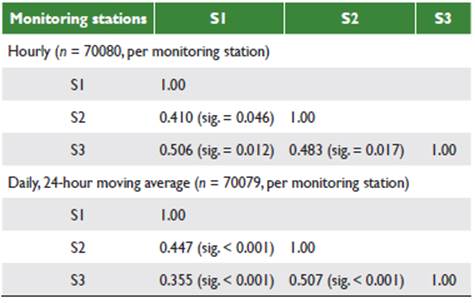
A Spearman's correlation analysis for all monitoring stations showed positive relationships with a tendency for medium values, Spearman's rs between 0.355 - 0.507. The results also showed uniform behaviour in the daily cycles of PM10 emission from motor vehicles and industries located across the entire study area. On average, S1 displayed the highest daily PM10 concentrations with daily concentrations of 115% and 146% higher than those displayed in S2 and S3, respectively.
Air quality standards
An initial assessment of daily PM10 concentrations was conducted in relation to the public health risk limits established by Colombian legislation (MAVDT, 2010) and WHO (2005) for a 24-hour exposure time. The results showed that S1 station was the most critical from a public health viewpoint. This monitoring station exceeded the Colombian daily limit 31% of the time during the study period, but especially during the month of February, where the average daily PM10 concentration was 107.8 µg/m3 (Figure 3). During that month, the daily legislative limit was exceeded 54.1% of the time. In contrast, the daily PM10 concentrations recorded at the S2 and S3 stations complied with the Colombian limit 99.5% and 100% of the time during the study period respectively. According to the daily limit established by WHO, the results showed on a monthly average that PMl0 concentrations in the S1 and S2 stations represented a public health risk during all months of the year (PM10 > 71 µg/m3) and in February (PM10 = 52.2 µg/m3), respectively. The monitoring stations S1 and S2 exceed this daily limit 92.7% and 31.7% of the time during the study period. S3 station showed the lowest public health risk. This station exceeds the daily limit 13.0% of the time during the study period.
The order of precedence established by quartiles (Q) to assess the risk per daily exposure to PM10 showed on average that the first three months of the year were Q1 in all monitoring stations. February was highlighted as the highest risk for public health, followed in order of precedence for the months of March and January (Figure 3). In contrast, the Q4 months or lowest risk for public health were in order of precedence July, June, and August. A similar monthly trend was observed for all monitoring stations during the study period.
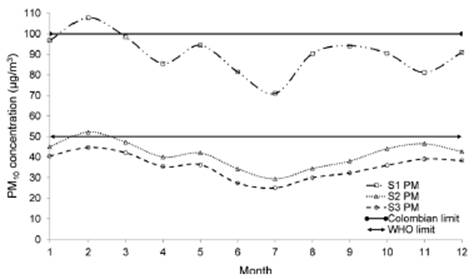
Figure 3 Average daily PM10 concentrations at the monitoring stations (S1, S2, and S3). Month: 1 = January, 2 = February, 3 = March, 4 = April, 5 = May, 6 = June, 7 = July, 8 = August, 9 = September, 10 = October, 11 = November, 12 = December. PM = PM10 concentration
During the month of greatest risk to public health (February), variations in the concentration of PM10 between the days of the week concerning legislative limits referenced for an exposure time of 24 hours were studied. On average, the results showed that at station S1, PM10 concentrations represented a health risk during most days of the week in relation to the Colombian limit, except for the period of exposure between Sunday and Monday (PM10 = 96.2 µg/m3). The previous trend was similar at station S1 and S2 from the daily limit established by WHO (Figure 4). On average, station S3 was the only one that complied with the legislative limits referenced in this study during February.
Atmospheric condition
The prevailing AC for stations S1, S2, and S3 between 6 - 18 hours (daytime) was slightly unstable (AC = 4; occurrence frequency for 24 h, f-24 h = 19.5%), unstable (AC = 5; f-24 h = 22.7%), and unstable (AC = 5; f-24 h = 24.5%), respectively. As for the prevailing AC between l8 - 6 h (night time), it was stable (AS = 1): 35.0% (f-24 h), 50.0% (f-24 h) and 49.2% (f-24 h), respectively. On average, for the entire study area, the results indicated that the prevailing AC during the daytime (6 - 18 h) was slightly unstable and unstable (AC between 4 and 5.5; f-24 h = 46.1%). At night time (18 - 6 h), the prevailing AC was stable (AS = 1; f-24 h = 45.1%). A Kruskal-Wallis test for stations S1, S2, and S3 showed that there were no significant hourly variations in AC (p-value = 0.827). In other words, there was similar behaviour in the hourly AC during the study period for all monitoring stations. Figure 5 shows the average hourly AC during the sampling period from the quantitative scale used in this study.
Figure 5 Average hourly AC at the study areas (S1, S2, and S3). AC: 1 = stable, 2 = slightly stable, 3 = neutral, 3.5 = neutral to slightly unstable, 4 = slightly unstable, 4.5 = slightly unstable to unstable, 5 = unstable, 5.5 = unstable to very unstable, 6 = very unstable. PM = Average hourly
However, on an average monthly basis the results showed comparatively that the order of precedence for the degree of daytime atmospheric instability was as follows: S3 (AC = 5.5) > S2 (AC between 5 and 5.5) > S1 (AC between 4 and 5). The results also showed that the order of precedence for PM10 concentration was as follows: S1 (90.2 µg/m3) > S2 (4l.3 µg/m3) > S3 (35.6 µg/m3).Thus, the results indicated that the daily PM10 concentrations were the lowest at the monitoring station that associated the highest degree of daytime atmospheric instability (see S3 in Figure 6).
Figure 6 Monthly comparison between PM10 concentration and daytime atmospheric stability. Month: 1 = January, 2 = February, 3 = March, 4 = April, 5 = May, 6 = June, 7 = July, 8 = August, 9 = September, 10 = October, 11 = November, 12 = December. AC: 1= stable, 2 = slightly stable, 3 = neutral, 3.5 = neutral to slightly unstable, 4 = slightly unstable, 4.5 = slightly unstable to unstable, 5 = unstable, 5.5 = unstable to very unstable, 6 = very unstable. PM = average daily PM10 concentration
Discussion
Urban PM10 pollution
On an hourly and daily basis, the results suggested a similar trend in PM10 concentrations between all monitoring stations (Spearman's rs between 0.355 - 0.507; see Table 2). This trend was associated with the uniform behaviour in the PM10 emission cycles by mobile (vehicles), fixed (industries), and natural sources in the study areas. The monitoring stations selected in this study covered 21.9 km (in a straight line) with relation to the 33 km length of the city, from north to south. Therefore, the results suggested that this uniform trend in PM10 emission cycles per hour and per day was probably similar in all sectors of the city of Bogotá.
On an hourly timescale, the results allowed us to identify the most critical time interval for PM10 from the point of view for urban public health. On average, this time interval was from 6 - 11 a.m., with the maximum PM10 concentrations between 8 - 9 a.m. (Figure 2). Thus, public health surveillance and control agencies should establish guidelines for sensitive population groups (children and older adults) during these time periods. For example, there should be a restriction of outdoor physical activities at educational institutions for children - especially around the monitoring station S1, where the average hourly PM10 concentrations were 115% and 144% higher in relation to that observed at S2 and S3, respectively.
The reference legislation made it possible to demonstrate that the most critical monitoring station within the public health framework was S1. On average, this station exceeded the Colombian daily limit (24-h exposure time) during February by 7.8%, and the WHO daily limit for all months of the year by 80.4% (Fig. 3). Based on the WHO Air Quality Guide (WHO, 2005), the daily PM10 concentration observed in February at the S1 monitoring station (average = 107.8 µg/m3) could increase the short-term mortality rate by 2.9% with relation to the mortality rate observed for a concentration of 50 µg/m3 (WHO maximum permissible level). The WHO (2005) reported that the adverse effects on human health could not be ruled out below the established maximum permissible level, but that compliance with these standards supposes a significant reduction of the risks on public health. On average, for all months, in the area of influence around the S1 monitoring station, there was probably an increase of 2.0% in the daily mortality rate associated with PM10. S2 and S3 monitoring stations complied with the Colombian limit during all months, and the S3 station was the only one that complied with the WHO limit throughout the year.
The order of precedence established by quartiles to assess the monthly risk for exposure to PM10 in Bogotá was as follows: Q1 (February > March > January), Q2 (May > December > October), Q3 (November > September > April), and Q4 (August > June > July). On average, during the Q1months the daily PM10 concentrations were shown to be 11.5%, 16.8%, and 35.9% higher than those observed in the Q2, Q3 and Q4 months respectively (Figure 3). In the present study, the results suggested that public health surveillance and control agencies should plan and implement different strategies according to the monthly Q value. For example, there should be more demanding strategies of PM10 control and surveillance during the months of greatest public health risk (Q1) in comparison to the months of lowest public health risk (Q4). On average, the short-term mortality rate during the Q1 months could be increased by between 0.46% - 1.32% with relation to the short-term mortality rate of Q4 months. This was based on an increase in the short-term mortality rate proposed by WHO Air Quality Guide (WHO, 2005).
Additionally, variation of the PM10 concentration during each day of the week for the most critical month (February) was evaluated from all monitoring stations. On average, the results showed an increase in daily PM10 concentrations as the week progressed, reaching its maximum level during the exposure period between Thursday and Saturday (Figure 4). PMl0 concentrations during this exposure period exceeded the Colombian daily limit at station S1 (15.6%), and the WHO daily limit at the stations S1 and S2 (S1 = 131%; S2 = 12.9%). Monitoring station S3 complied with all legislative limits of reference. A similar trend was observed in daily PM10 concentrations for other months. Therefore, the results suggested that this exposure period is the highest risk during the week in relation to the possible PM10 impact on human health.
On a weekly basis, the highest daily PM10 concentrations tended to occur during the exposure period between Friday and Saturday (Figure 4). On average, concentrations during this exposure period were higher (S1 = 14.3%, S2 = 13.3%, and S3 = 16.8%) compared to the concentrations observed during the exposure period between Sunday and Friday. This trend was probably due to the fact that in Bogotá there was a restriction on vehicular movement due to traffic congestion from Monday to Friday. This traffic restriction prevented the use of 40% of the city's vehicles between 6 and 9 a.m., and 3 and 7 p.m. In other words, there was no traffic restriction on Saturdays; which probably explained the increase in PM10 concentrations on this day.
AC influence
With relation to the influence of AC, the results showed the best possible scenario from a public health viewpoint for maximum hourly PM10 concentrations. Namely, the maximum concentrations recorded by the monitoring stations S1 (135 µg/m3), S2 (62.4 µg/m3) and S3 (52.3 µg/m3) occurred during daytime periods (8 - 9 a.m.), when the prevailing AC was between unstable and very unstable (Figure 5). This suggested high PM10 dispersion and a probable reduction in hourly concentration during these extreme air pollution episodes. Otherwise, the maximum PM10 concentrations in Bogotá during daytime would probably have been higher.
The results showed that during night time the prevailing ACs were stable (AC = 1). This suggested a low PM10 dispersion during these time periods and therefore a probable increase in hourly concentrations. Again, the best possible scenario in the public health framework for monitoring stations S1 and S2 occurred given that during night time periods the lowest hourly PM10 concentrations were observed (Figure 5). On average, night time PM10 concentrations at monitoring stations S1 and S2 were 20.1% and 4.61% lower than those observed in daytime. However, hourly PM10 concentrations at the S3 station were different. On average, at this monitoring station, the night time PM10 concentrations were 1.39% higher than those observed in daytime, despite a probable decrease in the emission sources of PM10 such as traffic and industries. The results suggested that the increase in night time PM10 concentrations at station S3 was probably associated with the prevailing ACs, which were stable (low PM10 dispersion). Lee et al. (2013) and Vecchi et al. (2007) reported a similar trend under prevailing conditions of night time atmospheric stability (AC = 1) in the cities of Seoul (Korea) and Milan (Italy).
From the above, the analyses showed the hourly variation of PM10 concentrations between monitoring stations using station S3 as a reference, and considering that this monitoring station tended to show the highest degree of atmospheric instability in the daytime (S3, AC between 5 - 5.5; S2 and S1, AC between 4 - 5.5). The results showed that during the night time there were no differences between monitoring stations in the hourly AC (AC = 1). Hourly PM10 concentrations at the S1 and S2 monitoring stations were 144% and 13.3% higher than those observed at S3 station (Figure 5). Additionally, at this last monitoring station there was less difference between daytime and night time concentrations of PM10 (difference = 1.39%) in comparison with the monitoring stations S1 (difference = 20.9%) and S2 (difference = 4.61%). This trend was also supported by a lower hourly variation than the average PM10 concentrations at monitoring station S3, evaluated by the standard deviation (S3, o = 6.27 µg/m3; S2, o = 8.18 µg/m3; S1, o = 17.8 µg/m3). Thus, the results suggested that the monitoring stations located in urban areas where there were atmospheric conditions of greater instability tended to show lower concentrations and variations of hourly PM10.
Daily PM10 concentrations showed a trend like that described above for hourly PM10 concentrations. Monthly, the results showed, on average, that the daily PM10 concentrations were lower in the monitoring station associated with the highest degree of atmospheric instability (S3). The order of precedence in the degree of atmospheric instability for monitoring stations was as follows: S3 > S2 > S1 (Figure 6). The order of precedence for daily PM10 concentrations was as follows: S1 > S2 > S3. Results suggested an inverse relationship between PM10 concentration and atmospheric instability.
Finally, in the present study, a relationship was observed between atmospheric instability and the type of land surface coverage (LSC). The results showed that urban areas of greater atmospheric instability (lower PM10 concentration) were characterized by a predominantly vegetated LSC (S2 = 86.2%; S3 = 74.6%; see Table 1). In contrast, urban areas of lower atmospheric instability (greater PM10 concentration) were associated with a predominantly impervious LSC (S1 = 68.9%). Studies in urban areas have reported a significant influence of a vegetated LSC on PM10 concentrations. For example, Chen et al. (2015) found that the presence of trees in Wuhan (China) reduced PM10 concentrations from between 7% - 15%. Similarly, Shan et al. (2007) and Islam et al. (2012) reported a reduction of total suspended particulates (<100 µm) in urban areas by 30% (Shanghai, China) and 55% (Khulna, Bangladesh), respectively. A vegetated LSC also acted as an effective sink for gaseous and particulate atmospheric pollutants (Fowler et al. 2004).
Conclusions
The results suggest that public health surveillance and control agencies should pay more attention to urban sectors with lower atmospheric instability, because these urban sectors show higher concentrations (between 131% - 144%) and variations of PM10 compared to urban sectors of greater atmospheric instability. On average, urban sectors with lower atmospheric instability show an increase in the daily mortality rate of 2.0% with relation to the mortality rate for a daily PM10 concentration of 50 µg/ m3 (WHO limit). According to WHO (2005), an increase in the daily mortality rate of 5% requires immediate corrective measures. The type of urban LSC can probably be used as a public health indicator, since in urban sectors where there is evidence of greater increases in the daily mortality rate by PM10 (lower atmospheric instability), an impervious LSC predominates instead of a vegetated LSC.
Finally, the findings of this study serve as a reference point to deepen our knowledge about the behaviour of PM10 concentrations and the influence of AC, allowing us to develop and implement different strategies of surveillance and control for public health in megacities. However, the following limitations form part of this study, requiring further attention. First, the number of years for the PM10 time series (six years) was limited due to LSC changes in the areas covered by the monitoring stations; for analysis of the influences on the AC upon PM10 concentrations, the same LSC distribution is required throughout the study period. Second, the monitoring stations do not have similar characteristics regarding the distance and emission intensity of the PM10 sources (highways and industries). Third, PM10 concentrations and AC for the entire study area are evaluated using data from only three monitoring stations, so the number of stations could be increased.

