


 English (pdf)
 Article in xml format
 Article references
 Send this article by e-mail
 Cited by SciELO
  Cited by Google
  Similars in
SciELO
Similars in
SciELO  Similars in Google
 Permalink
For the determination of coverage there are patented methods such as the calculation of the received signal strength indicator (RSSI) by positioning based on the propagation of the frequency hopping of the spread spectrum, which reduces the effect of multi-channel interference, obstacle blocking, and multi-path effect by implementing a MinMax positioning algorithm (Zeng, Xiao, He, & Yu, 2017).
Similarly Rademacher and Kessel (2015) establish the characteristics of power evaluation using three mathematical methods to check empirically the behaviour of the received power which has a normal probability distribution, using the libpcap software library and the power of the spectrum through the fast Fourier transform.
The proposal of Chen and Zhan (2017) allows a spectrum monitoring system to use a real time application that can find the RSSI intensity of the radio bases by means of the positioning algorithm with the help of statistical methods of maximum probability (Yaghoubi et al., 2014), as is the case with mobile cellular networks, spectrum measurement devices are classified into three categories: (a) spectrum analysers, (b) test drivers and (c) instruments dedicated only to cellular technology; for this purpose many monitoring stations require to know the input power in the receiving equipment from the measurement results as they show it (Salvadè et al., 2004). In addition, measurement standards must be established according to the technical standards established by the (ITU, 2015) for spectrum monitoring.
For the study of Wireless Network coverage (WLAN) there are different positioning techniques according to the classification made by Yassin and Rachid (2015) including the Cell-ID, time, RSSI and angle; for the particular case being studied a system characterization was made by means of the Cell-ID method in order to identify the power level of the nearest access point, and the RSSI in order to quantify the real power of a received wireless signal, which is subject to losses in free space and phenomena such as attenuation, reflection, diffraction and dispersion according to (Kochláñ et al., 2014).
The research compares different methods of RSSI signal level capture (Yassin & Rachid, 2015) to process the information of the frames stochastically every I0msg, through the embedded wireless cards or dongle that perform a pre-processing of the captured records by means of non-linear regression algorithms to obtain an adequate propagation model.
By analysing the packet structure in Wi-Fi MAC (Bhanage, 2017) using the aggregation effect, multiple packets are combined and transmitted independently in a single transmission unit via the MAC service data units (MSDU) to the Internet Protocol (IP) stack in order to access the frame structure (Bhanage, 2017).
Related work
Generally, a Radio Frequency (RF) propagation model consists of predicting the coverage of the signal according to the power level in order to plan the network based on measurements or simulations, as represented by Malik et al., (2014) with the Opnet Modeler software that makes predictions by analysing the structure of the packets and fragments of the frames using the Markov chains.
Similarly, the calibration software patent of the radio propagation model of Ayadi et al. (2017) uses the field strength of the radio and the respective location data, applying the modified Newton's second order gradient that helps model the power intensity; this is a reference for the implementation of the research methodology proposed in the mitigation of errors in the design of the application.
Also Bouleanu et al., (2016) determines the prediction of a microwave system by means of the Radio Mobile application through simulation which compares the measurements made in multiple locations in order to find the correlation coefficient between the simulated and measured signal power values, using the irregular terrain model of two point-to-point rays (ITM). In the case of Hamim and Jamlos (2014), they compare the field strength measurements taken by a portable spectrum analyser and with the results they perform the simulation with the coverage models: ITM, ITU-R P.I546 and the Hata-Davidson empirical model in order to exhibit larger errors over longer distances and introduce the necessary corrections to increase the accuracy of the prediction.
According to Neidhardt et al., (2013) there are crowd-sourcing Android applications available which measure the performance of the network under the parameters of received power, latency, and performance, as well as determining a mathematical modelling of the measurements in place for frequencies in 2.4 GHz; however, they do not perform real-time processing.
On the other hand, Kasampalis et al., (2014) compare the results of the measurement campaigns by using simulations conducted with Radio Mobile and the ICS Telecom software, estimating the reception losses by using three empirical propagation models: NTIA-ITS Longley Rice, ITU-R P.1546, and Okumura- Hata-Davidson.
Design methodology
Based on the need to perform the measurements of the spectrum in an automated way, an application is designed to autonomously configure measurement parameters, capture, processing, mathematical and statistical analysis for the visualization of results, and the generation of an empirical-experimental analytical model as described below.
A. Functional analysis of the application
The processes, elements and activities are defined and identified, as well as the technical requirements of the work environment, user requirements and functional requirements. The synthesis of how the project is conceived is shown in figure 1, and the software architecture describes all the phases of the development of an application as described by Medvidovic and Taylor (2010).
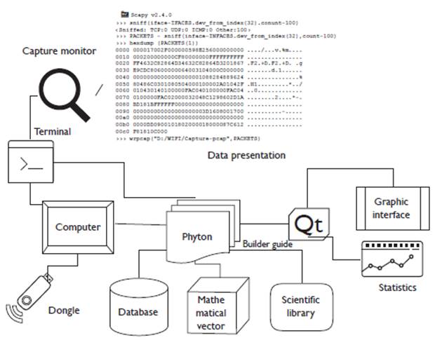
With the use of an internal or external wireless device working on the 2.4 GHz frequency, the spectrum scan is performed to capture the 802.11 standard frames by means of the computer; for this, the card is established in monitor mode using the physical interface to initiate the capture and administration of the native packages with the help of the Scapy application according to Zhou, Jacobsson, Uijterwaal, and Mieghem (2010) and the Network Driver Interface Specification (NDIS) controller that performs the driver function in the network interface card (NIC), enabling TCP / IP protocols (Rosati, 2014). Internally random channel jumps are made to determine the channel to analyse, and then the data is extracted from the structure of the beacons frames in order to perform the analytical processing that is visualized in the graphical user interface (GUI), the statistical results, graphs, equations and the models of propagation referenced (Sati & Singh, 2014).
B. Design of the programming structure
A structural scheme of the development of the application is established where the characteristics of the functionality of the algorithm and the logical design are synthesized, as shown in Figure 2.
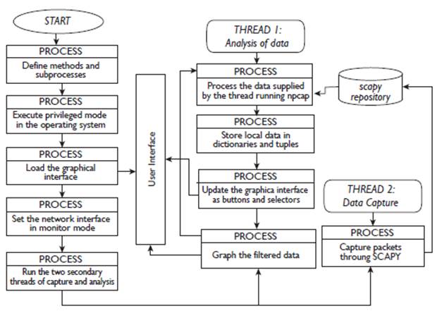
Initially the methods used in the application are defined, then the console or terminal is used to establish the network card in monitor mode accessible to the user (Günther et al., 2014) in order to capture the control and management frames within the header of the link layer and the resources of the operating system, on which the application is running. Next, the graphic interface is loaded where two programming threads (subprocesses) are started simultaneously, one for data analysis and the other for the capture of the beacos frames.
The capture is carried out with Scapy using the "sniff" command and the local variables are routed in the RAM memory, which are simultaneously accessed by the "data analysis" thread. In this subprocess, the data supplied by the Scapy library is managed to create the payload (Robyns et al., 2015), where local data is stored in dictionaries and tuples (Giustiniano et al., 2015). Later the graphic interface is updated with the information of the found networks along with the power and other data that contains the beacons frames, and finally the data is filtered and graphed for the application.
C. Development of the application
In the research, the Python development tool was based on the guidelines of Lei et al., (2015) for programming and accessing information at the physical layer, air interface and link level, because it facilitates low-level programming and optimization of physical resources as expressed by Zou et al., (2017) and Guerrero-Higueras et al., (2013);
with Npcap, the hardware is established in monitor mode, and with Scapy (Rodofile et al., 2015), the capture is executed from the wireless physical interface in a text file with extension .pcap, which contains the extracted data in real time. The tools mentioned above are integrated with the Pyqt5 application (Harwani, 2018) for the presentation and visualization of the graphic interface designed.
D. Installation and Implementation of graphical interface
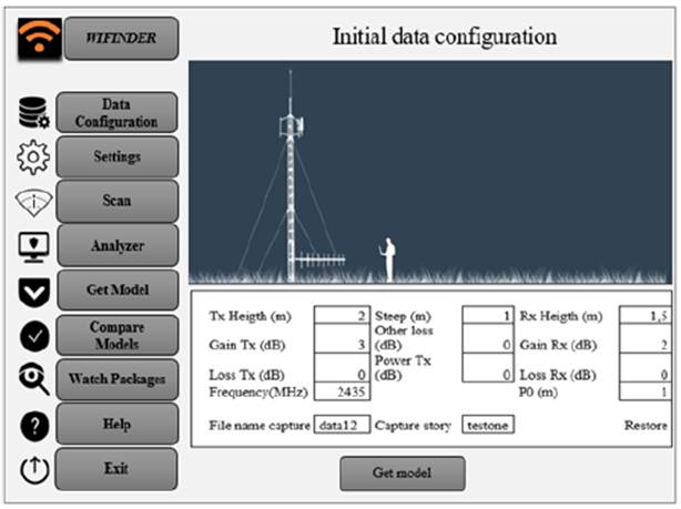
A friendly graphical interface is installed with the elements multimedia, icons, indicators and tables in real time in a graphic, graphically linking the mathematical processes and the data obtained statistically as shown in Figure 3.
In the evaluation and validation stage of the application, the pilot tests are executed to obtain the databases of each one of the tested measuring points which are tested in the working frequency of the designed application.
Data configuration
This is the process where the adjustment of the parameters of the environment and the system are made by selecting the text boxes of the elements such as the height of the transmitting antenna, the power, the gains and the losses in transmission, the frequency, other losses, the receiving antenna height, the gain and loss in reception, the initial position of the receiver, and the name of the directory that stores the records along the path (Bureau, 2011), as shown in Figure 3.
Setting interface
The NIC configures the channels to be analysed, the number of samples that are required, and the sampling time according to the technical specifications using Scapy Iface libraries (Scapy, 2018). For the case study, samples are taken every 40A, Pinnagoda, (2017) suggests taking dimensions of a few hundred meters so that the path profile and the general environment of the receiver do not undergo significant modifications as recommended (Recommendation P-1406-2 ITU-R, 2015).
Data Capture
When running Scapy in the background using the Ifaces command as proposed by Chen et al., (2017), the capture of the data in the active interface of the power levels and other data to be processed of all the active networks that emit the beacons frames is initiated, this happens when "scan" is selected in the menu (Sandhya et al., 2017).
Data analysis
This is the selection process of the network to be analysed; for this the "analyser" menu is chosen, where the data is filtered by MAC or by name of the network, the graphs with the RSSI values in dBm, and the basic statistics (average, modest, variance, standard deviation, minimum and maximum) of each of the measurement points in the path are automatically displayed.
Obtaining the model
The "get model" button generates the analytical semi-empirical propagation model as seen in Figure 4.
The measurements are carried out continuously under normal environmental conditions and on similar days to maintain the accuracy of the thereof (Ponomarenko-Timofeev et al., 2016). The samples are taken at 3-minute intervals; when the last sample is taken, the program is instructed to generate the mathematical equation.
Comparison of models
With the "compare models" button option, the comparison between the mathematical models obtained by the application against models (Erceg-Sui, Minimun Squares, Okumura-Hata and Cost-231) is visualized, as shown in Figure 4.
Results and discussions
In radio propagation studies it is important to consider the coverage of wireless radio systems according to the technical characteristics of the equipment; however, external factors and environmental conditions are often not considered, therefore, a prediction of the power levels is used. Thus, parameters that can describe the behaviour must be obtained, as is the case of the loss coefficient (n) obtained empirically and the statistical error parameter (k) (Morocho-Yaguana et al., 2018), applying Levenberg Marquardt Algorithm (ALM) as a method of solution according to the equation 1 (Kaveh et al., 2017).
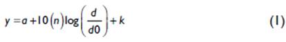
Assuming that: a is the trajectory losses at a reference distance, n the exposure of losses, d the distance of each measurement, d0 is the reference distance, and k is the error of sensitivity of the random effects.
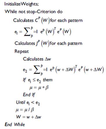
The optimization function "scipy.optimize.curve_fit" obtained from (SciPy v1.2.1 Reference Guide, 2018) is used, which makes an adjustment through the ALM within the programming by means of Phyton with their respective libraries (Forsyth & Zarrouk, 2018). The ALM analysed by Cui et al., (2016) is a combination of maximum descent methods and the Gauss-Newton method that exhibits rapid convergence (Cornejo & Rebolledo, 2016).
Internally, the ALM performs the weight adjustment of the positional uncertainties of each point of the samples obtained, using the estimation of the error k within a variance and covariance matrix.
If the ALM compared with the standard least squares method, by using (2) to minimize the sum of the squares of the deviations between the measured power values and the prediction values with the model as a solution, minf (x), toxe ∈ R;.
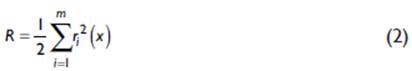
It is observed that, the vector of the residues is r(x):
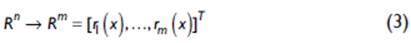
and each cada r(x), i= I.....m, for m >= n, as a non-linear function of Rn in R.
By applying equation 2, the corresponding curve is obtained as shown in Figure 4, which in analytical terms is generated by the software in real time and equation 4 is obtained:

Otherwise it happens when applying Levenberg-Marquardt's algorithm as interpreted by Toushmalani et al. (2014) as observed in figure 5, which allows us to generate the parameter of the sensitivity error of the deviations of the power values with respect to the distance and the exponent of losses of the environment under measurement, with this algorithm a better precision is achieved (Newville & Stensitzki, 2018) and it is represented as a result in equation 5.
The results of the obtained parameters are expressed according to:

When confronting the semi-empirical model obtained with the propagation models Okumura-Hata and COST 231-Hata; it is observed that the Okumura-Hata model is based on measurements for mobile macro cell systems, for distances between the mobile and the base station between 1 and 20 kilometres. Define the expressions for four different environments, urban dense and urban medium, suburban and rural; for the case of the urban environment, it uses the general equation (6) for losses, where Lurb (dB) are the decibel losses using the expression of Yacoub (2019).
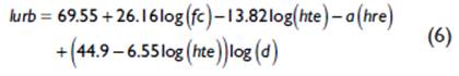
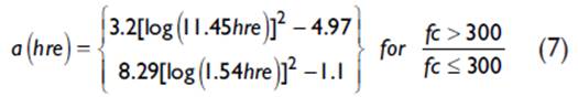
Where fc (MHz) is the operating frequency, hte (m) is the height of the transmitting antenna, d is the distance between the base station and the mobile station, and a(h re ) is the correction factor of the receiving antenna. The calculation of this factor depends on the density of the environment and is calculated with (7):
In the case of the Model Cost 231-Hata (Ambroziak & Katulski, 2014), the conditions of use are based on the characteristics of frequencies between 1500 to 2000 MHz, mobile height between I and I0 m, height of the base station between 30 and 200, my link distances of 1 and 20 km, c is 3dB for urban areas (Stüber, 2017). The resulting basic losses are represented by (8):
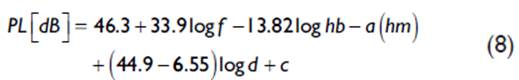
Where hb is the height of the base station, hm is the height of the mobile, a(hm) is the correction factor of the height of the mobile, for urban area it is obtained with (9):

Checking with the Erceg-Sui model (Elsheikh et al., 2017) which uses equation (10), it works in frequency ranges from 2 GHz to 11 GHz, proposes to characterize scenarios by categories according to the following parameters: d is the distance between base and receiver in meters, À is the wavelength, y is the exponent of losses, hb is the height of the base station in meters, s is the shadowing effect and a, b, c are constants that depend on the category of the terrain (Choudhary & Dhaka, 2015).
According to Figure 4, in terms of received powers, the LVM loss model is the best fit for field measurements of tabulated mean data compared to the normal least squares model with a margin between 2dB and 4dB difference.
When confronted with the Okumura-Hata model there is a considerable loss between 10 dB to 14 dB below the value obtained with the LVM model for each measured power point, which means that this model does not fit the power prediction techniques; likewise, it can be inferred that Cost-231-Hata and Erceg-Sui models are also not good predictors due to the number of variables that have to be considered in a field study; it is convenient to establish a correction factor in the analytical expression obtained in order to determine that the power probability does not exceed the reception threshold limits at the time of performing the test drive on the radiated power levels of the transmission equipment.
Conclusions
The environmental conditions of the real time field tests are established in an environment with similar characteristics regarding: measurement times, climatic conditions, computing capacity, sampling, equipment calibration, errors and possible dispersing elements in the LOS and NLOS links in urban environments.
For greater safety, the locations of measurement points on shorter paths must be estimated according to the wavelength, strictly respecting technical regulations for spectrum measurement and the operating conditions of the measurement equipment.
Test drive measurements should be selected so that there are no objects that produce reflections and generate discontinuities in the measurements. Direct examination of the ground profile is required in a complete and accurate manner, guaranteeing a confidence interval of 3 dB around the real average value measured in the field, and ensuring a higher level of power and a decrease in the sensitivity error resulting from random effects (k) obtained in the model equation.
The Python and Scapy software tools used speed up the capture of 93% of the frames beacons transmitted in the wireless channel by continuously sampling the power levels every I0 milliseconds, so there is a random channel hop, in turn facilitating the processing of the spectrum signals more accurately.
The source code in Python allowed only three programming threads to integrate the lines of code in a compact way to reduce the processing time: (1) the main thread that controls the graphic interface to manage the events and threads, (2) another thread that captures the frames and stores the variables, and (3) the final thread that processes the frames for the statistical analysis of the data, applying the ALM algorithm and visualizing the equation in the graphic interface.
When the ALM algorithm is used, the fit of the data with the non-linear least squares problem is improved, since it is an iterative algorithm that combines two methods to facilitate the convergence of the value of the power levels and reduces the processing time of the estimated parameters.
One mechanism for improving the application in the future is to use artificial intelligence algorithms, such as "Reinforcement Learning" to reduce sampling times under extreme environmental conditions.
Another way to optimize the software is to use an optimal overfit prediction model through Machine Learning, using a large data set for training with cross validation and early detection techniques, which increases iterations and reduces redundant data.

