


 English (pdf)
 Article in xml format
 Article references
 Send this article by e-mail
 Cited by SciELO
  Cited by Google
  Similars in
SciELO
Similars in
SciELO  Similars in Google
 Permalink
Introduction
At the international level, the importance of hydrocarbons could hardly be overstated and, in the case of Mexico, it has come to play a preponderant role in the economic, politic, and social arenas. Modern exploitation started in the mid-19th century and in 1938, after almost one century and thanks to several developments, a most relevant event took place: President Cárdenas nationalized the petroleum industry, and PEMEX was created as a government monopoly to handle every aspect of hydrocarbons exploitation, from exploration and extraction to refining and distribution.
After an uneven evolution, by the 1980s the Mexican petroleum industry had become a world power. Mexico was the fifth country with the largest production and held 8.2% of world reserves; petroleum contributed 18% of the Mexican GDP, and more than 90% of primary energy generation. Regarding government income, during almost the last three decades, hydrocarbons contributed an average of 32% with a peak of 44% in 2008; after the petroleum reform of 2013, that percentage dropped to 13% in 2015 (Hernández, 2017).
Therefore, this research is concerned with a quantitative appraisal of this decrease, in terms of an increase in income taxes that should be implemented in order to compensate for the loss and allow the government to maintain its budget. To this end, we build a Social Accounting Matrix (SAM) and design an Applied General Equilibrium Model (AGEM) with the main objective of assessing household's welfare loss.
As far as we know, no research on the specific issue of taxes on hydrocarbons has been carried out using this methodology, although a good deal of AGEMs have been developed and validated on energy topics (Bhattacharyya, 1996; Beckman, Hertel & Teyner, 2011). Also, according to a recent paper published by Transportation Research: "Computable general equilibrium (CGE) models are an increasingly popular method for assessing the economic impact of transport, including both direct and wider economic impacts, as they can determine the distribution of impacts among every market and agent in the economy by simulating the behaviour of households, firms and others from microeconomic first principles. Aside from their traditional role estimating changes in macroeconomic variables, CGE models can provide a measure of welfare that guarantees no double counting and accounts for nth order effects" (Robson, Wijayaratna & Dixit, 2018). The same applies to our case and to any other application of CGE models.
In the first part of this paper, we build a Social Accounting Matrix of Mexico for 2008 (SAM-Mx08). We start from the input-output table of Mexico for 2008 (IOT-Mx08), prepared by the National Institute of Statistics and Geography (INEGI). House are disaggregated based on results from the National Survey of Households' Income and Expenditures (ENIGH08). The information is complemented with several additional sources.
It is worth noting that the SAM is not only a database to carry out Applied General Equilibrium (AGE) analysis, but also a valuable result in itself, since it provides a comprehensive and detailed vision of the Mexican socio-economy. More importantly, it is possible to apply a wide range of analytical methods to obtain a better understanding of the economy.
In the second part, we design an Applied General Equilibrium Model (AGEM-Mx08), robust and parsimonious, of general application; that is to say, we believe that this AGEM could also be modified and applied to a wide range of economic issues (environment, energy, trade, etc.).
Finally, in the third part we implement an application of the AGEM to the specific case of taxes on the extraction of hydrocarbons. This is of great socio-economic importance, given their high participation in the financing of public services such as education and health.
By the above, we consider that this work contributes substantially to generate (and to enable the generation of) knowledge about Mexican socio-economy to sustain social development and the construction of public policies of national scope. The paper ends with section four, dedicated to our main findings and final comments.
Social Accounting Matrix of Mexico for 2008 (SAM-Mx08)
To build the SAM-Mx08, we follow the conceptual framework developed by several authors (Bellú, 2012; Breisinger, Marcelle & Thurlow, 2010; Defourney & Thorbecke 1984; Keuning & Ruijter 1988; Miller & Blair 2009; Müller, Pérez & Gay, 2009; Thiele & Piazolo, 2002; Yusuf, 2007). For the case of Mexico, we follow the work of Núñez (2008; 2004).
We start from the input-output table of Mexico for 2008, the domestic economy product-by-product of 19 sectors according to the North American Industry Classification System (NAICS) (Instituto Nacional de Estadística y Geografía [INEGI], 2013b), published in INEGI's site1, which we call IOT-Mx08; and develop the SAM with additional information from the Goods and Services Accounts (G&SA) (INEGI, 2010a), Institutional Sectors Accounts (ISA) (INEGI, 2010b), National Survey of Income and Expenditure of Households 2008 traditional (ENIGH08) (INEGI, 2009), and the 2008 Law of Income Tax.
Construction of the MCS - Mx08
To develop the SAM-Mx08 (in what follows the SAM) we follow as main criteria that of maintaining the structure of the economy implied by the IOT-Mx08 (in what follows the IOT), and that of achieving the greatest possible consistency with national accounts.
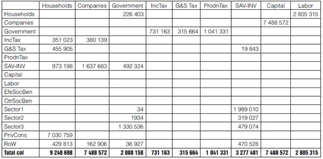
To begin with, we reorganize the IOT data to clarify how the accounts are structured, particularly the structure of value added (VA) and taxes. Table 1 presents the IOT, rearranged with the columns of the productive sectors as a succession of concepts whose sum leads to the total gross output (at basic prices) of each sector. For illustrative purposes, we use a version aggregated to three sectors: we add the first 4 sectors into Sector1, manufactures are Sector2, and the remaining sectors are lumped into Sector3. Then remuneration is disaggregated into the three components specified by the IOT: salaries and wages, effective social contributions, and other social benefits; Taxes on Production follow, and then the Gross Operating Surplus (GOS or Capital Rents). Unless otherwise noted, all figures are in millions of current 2008 pesos.
Table 1 MIP reorganized and aggregated to three productive sectors
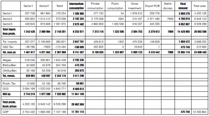
Source: Compilation based on the MIP (INEGI, 2013a).
With this, we can see production as a succession of added concepts. Let's consider the Sector1 column:
a) The sum of inputs from the three sectors is the total for domestic inputs (1 243 426).
b) Imports plus (net) taxes on goods and services plus the previous sum, amounts to total use for Sector1 (1 461 917).
c) The sum of wages and salaries, effective social contributions and other social benefits, amounts to total remunerations (638 083).
d) Gross value added (GVA) equals total remunerations plus taxes on production plus Gross
Operating Surplus (GOS) (2 743 218).
e) Finally, total output (at basic prices) is equal to the sum of Gross Value Added (GVA) plus total inputs (4 205 135). In a similar manner, we obtain total gross production for the rest of productive sectors.
f) Turn now to the fourth column (intermediate demand or inputs to production), which can be interpreted as an aggregation of all productive sectors: In the last row the total GDP at basic prices is precisely in the fourth column (11 781 115), and adding the total taxes on goods and services we obtain GDP at market prices (12 256 864).
g) The columns of final consumption are kept just as they are in the IOT, but we aggregate gross fixed capital formation and changes in inventories into a unique vector of gross investment.
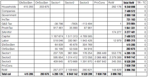
h) Once the IOT has been more conveniently reorganized, we proceed to use the conceptual framework referred to earlier to get the scheme of Table 2 (which we will refer to as the Macro-SAM), which consists, in principle, of 14 accounts: Companies2, Households, Government, Taxes on Goods and Services (G&S Tax), Taxes on Production (ProdnTax), Savings-Investment (SAV-INV), Capital, Labor, Effective Social Benefits (EfeSocBen), Other Social Benefits (OtrSocBen), the three Productive Sectors, and the Rest of the World (RoW).
Table 2 IOT data into the scheme of the Macro SAM. Part 1
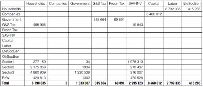
Source: Compilation with data of the IOT-Mx08 (INEGI, 2013a).
In Table 2, we see that the column for Households is that of Private Consumption in the IOT: G&S Tax (which include VAT), demand from productive sectors, and imports. The corresponding row contains income from Labor: Wages and Social Benefits.
Companies only have the Gross Operating Surplus (GOS or Income from Capital rents) transferred from the Capital account.
The public sector has three accounts: Government, Taxes on Goods and Services (G&S Tax), and Production taxes (ProdnTax). The last two collect taxes from Households, and transfer them to the Government which, so far, only spends on goods produced by sectors and by the RoW (Column of Government consumption in the IOT).
Then, the Savings-Investment account, which is the gross investment we have got from the OIT. And the Capital account, which is simply the capital rents generated by the economy (Gross Operating Surplus, GOS) as defined in the Mexican System of National Accounts.
Total remunerations have also three elements: Labor (wages and salaries), Efective Social Benefits (EfeSocBen), and Other Social Benefits (OtrSocBen), which are payments from productive sectors to workers; these payments are transferred to the Households account.
Next, we have productive sectors, which pay taxes, employ Capital and Labor, and buy inputs (domestic and imported) to generate production, which is distributed among intermediate demand (inputs) and final demand (private, public, investment and exports). Finally, the RoW obtains income from imports and spends in exports.
Up to this point, we have not introduced any new data, but just reorganized the numbers in the OIT according to the square format of the SAM, whereupon it is possible to add the total per column and per row, and to compare both: total revenues and total expenses.
The last column is the difference (income minus expenditure) for each account. Households, Companies, Government, Savings-Investment, and RoW, have non-zero differences because some elements are missing. For example, Households do not have income from Capital, nor from transfers; on the other hand, Households are not paying income taxes, and they are not saving. Since all the information of the IOT has been already included into the macro SAM, in what follows we resort to the system of national accounts, and to other sources to complete and balance the SAM.
To begin with, we open a new account for Income Taxes (IncTax), and include the figures given by the Institutional Sectors Accounts (ISA) (INEGI, 2010b), where Households (and Non-Profit Institutions that Serve Households) pay income taxes of 351 023, and Companies 380 139. The total revenue, 731 163, is transferred to the Government account.
Also according to the ISA, Companies' gross savings equal 1 637 683; Government saves 492 324; Households 973 198; and RoW (174 277), then total savings amount to 3 277 481. The RoW pays 12 979 to documented Labor, and transfers from the RoW to households (remittances from Non-Documented Labor) are 282 176 (283 778 - 1601). The Government pays to households social benefits other than social in-kind transfers (198 367), and other net current transfers (28 036), for a total of 226 403.
After we include this data in the SAM, opening at the same time another new account for Private Consumption (PrivCons), in which we place production for private consumption, we obtain a vector of differences between the total per row and the total per column, with a deficit for the Government of 935 815, a surplus in SAV-INV of 282 358, and a deficit for the RoW of 190 622.
The Statistical Discrepancy (SD) in Sector2 (Manufacturing) of 7909 is only 0.1% of total manufacturing. On the other hand, the RoW has a deficit of 190 622, while the ISA report for the RoW 197 464 Net Property Income. Therefore, we assume that SD is an additional amount of exports by Sector2, paid by the RoW, then Sector2 gets balanced.
With regard to the public deficit of 935 815, it happens that the Government is not receiving the levy corresponding to the Other Taxes on Production (OTP), which for some reason in the IOT have been aggregated to the Gross Operating Surplus (GOS). To separate the OTP from GOS, we draw on Table 58 of the Goods and Services Accounts (G&SA) (INEGI, 2010a), and subtract to obtain effective GOS and therefore OTP (Table 3)3.
Table 3 Other taxes on production and gross operating surplus unbundling
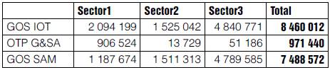
Source: Compilation based on the IOT-Mx08 (INEGI, 2013a) and G&SA (INEGI, 2010a).
After the inclusion of these additional data into the SAM under construction, the Government has a surplus of 35 625, thanks to the additional revenue from collection of the OTP. The RoW now has a deficit of 198 531, almost equal to its income from the net property (197 464). Then, we assume that the Government transfers its surplus to the RoW as Property Rent, and the rest (198 531 minus 35 625) is covered by Companies (162 906). Therefore, the RoW and Government accounts are also already balanced.
Companies have now a surplus of 5 307 844 and, since they have covered all their expenses, said surplus is transferred to Households as capital rents. With these changes, as expected, the difference between Savings and Investment, which was not spent on capital goods (282 358), appears as a deficit in Households' spending, which would be absorbing an excessive quantity of produced goods and services.
To correct this difference, according to the criterion of maintaining the structure of the IOT, we adjust production for private consumption and investment to the amounts given for such difference, namely 7 030 759 (= 7 313 116 - 282 358) for private consumption, and 2 787 111 (= 2 504 753 + 282 358) for investment. Calculations are presented in Table 4.
Table 4 Adjustment of investment and private consumption
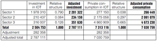
Source: Compilation based on the MIP (INEGI, 2013a) and CByS (INEGI, 2010a).
With these changes, all the accounts in the SAM are balanced, but as an effect of the adjustments, the following differences result in the productive sectors: 212 312 for Sector 1, -60 256 for Sector2, and -152 056 for Sector3.
In recent decades, multiple methods for balancing matrices have been developed: from simple programs, such as that of Zenios, Drud & Mulvey (1986) that minimizes a deviation function, to more sophisticated methods such as the cross entropy approach by Robinson, Cattaneo y El-Said (2000) (Debowicz & Golan, 2012; Temurshoev, Miller & Bouwmeester, 2013), which are used to ensure that the data are adjusted to balance the matrix under the fundamental idea that adjustment minimizes the change in the underlying structure of the economy.
In our case, we have arrived to relatively small differences (4.8%, -0.87% and -1.6% in the productive sectors), according to which, and to maintain the transparency of the data and the consistency with the system of national accounts, we consider that a manual adjustment is the most appropriate.
The adjustment is made as follows: from investment in Sector1 we subtract the difference 212 312, with which this sector is balanced. Then, to keep total investment at the same level (given by gross savings of 3 277 481), we add the same amount to investment in the other two sectors, weighted by their relative weight: 84 868 and 127 444 respectively. Finally, private consumption in sectors 2 and 3 is adjusted by the resulting difference: 24 612.
The matrix thus obtained is already fully balanced, as shown in Table 5.
Table 5 Balanced macro SAM-Mx08. Part 1
Source: Compilation based on the MIP (INEGI, 2013a) and CByS (INEGI, 2010a).
Disaggregation of Households
To elaborate a more complete and useful SAM for the analysis of economic issues, and, in particular, of public policies and their impact on the well-being of households, in this section we work a disaggregation of households, based on deciles as defined by the national survey of income and expenditure of households 2008 (ENIGH08) (INEGI, 2009).
In Table 6 we can see the income distribution in Mexico, according to the ENIGH08 (INEGI, 2009). The distance between the deciles with the highest and lowest revenue becomes immediately noticeable: decile X has more than 20 times more income than decile I, which gives an account of the deep distributive gap that exists in Mexico. In what follows, we use the classification by deciles in Table 6.
Table 6 Households total quarterly income
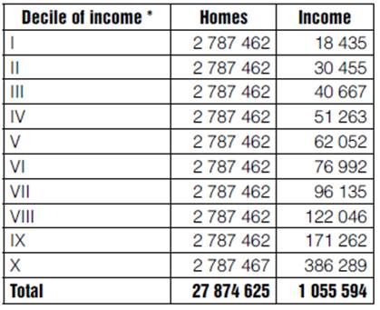
*Households organized by deciles according to quarterly total current income. Source: National survey of income and expenditure of the households 2008. Traditional. Table 6.2. (INEGI, 2009).
We start breaking down private consumption and respective taxes; calculations are presented in Table 7. We use the structure of the distribution of the total current expenditure, implied by data in Table 7.2 of the ENIGH08, and distribute the consumption and taxes weighing participation in each decile.
Table 7 Breakdown of consumption and taxes on goods and services
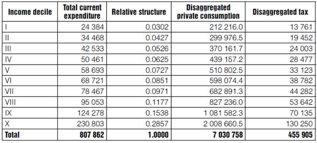
Source: Compilation based on the MCS-Mx08 and table 7.2 of the ENIGH08 (INEGI, 2009).
Now, to disaggregate the Income Tax we use the provisions specified by the Law on Income Tax of 2008 (DOF, 2007), stipulated by article 113. Table 8 contains the applicable provisions. In Table 9 we first calculate the tax paid by households with data from table 6.2 of the ENIGH08, and then distribute the taxes in the SAM on the resulting structure of relative participation.
Table 8 Income Tax on the monthly income of physical persons, 2008
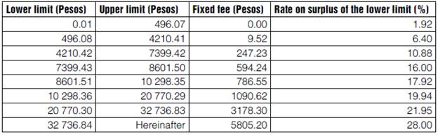
Source: Law of the income tax. DOF 01-10-2007.
Table 9 Breakdown of Income Tax by decile. Part 1
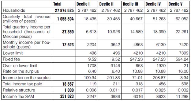
Source: Own elaboration, based on the ENIGH08 (National Households Income-Expenditure Survey 2008).
Table 9 Breakdown of Income Tax by decile. Part 2
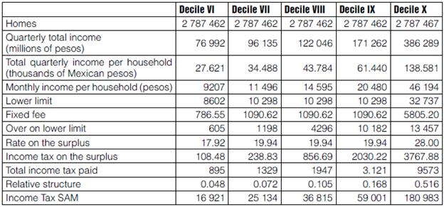
Source: Own elaboration, based on the ENIGH08 (National Households Income-Expenditure Survey 2008).
We continue with the breakdown of savings, using the same procedure followed for private consumption, but with the structure of the table 7.2 of the ENIGH08 deposits to savings, batches, saving, etc.
To end with Households' expenses, we disaggregate imports of households, based on the data of Table 5.2 of the ENIGH08 other miscellaneous expenses; calculations are presented in Table 10.
Table 10 Breakdown of direct imports by households
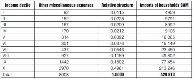
Source: Own elaboration, based on the ENIGH08 (National Households Income-Expenditure Survey 2008).
We now proceed to disaggregate the elements of households' income. Starting with Labor, we use the relative structure implicit in the data in Table 3.2 of the ENIGH08 to pay for subordinated work, we assume that these proportions are also applied to Social and Other Social benefits. Table 11 presents the estimates.
Table 11 Breakdown of payments to Labor
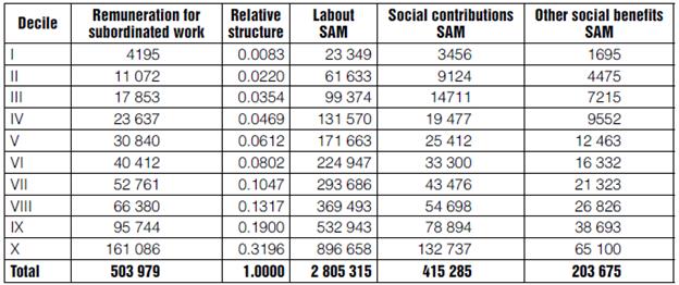
Source: Own elaboration, based on the ENIGH08 (National Households Income-Expenditure Survey 2008).
The following element is Government transfers, so we use data from Table 3.3 of the ENIGH08 benefits from government programs, in the same way as before for Labor.
We still have the RoW transfers, so we use the revenues from other countries from Table 3.3 of the ENIGH08, to disaggregate in the same way as we did before, using the relative structure.
Finally, the deficit between what was spent by each household and the revenues distributed so far, is necessarily contributed by income from capital (GOS). Whereupon, the SAM-Mx08, with 19 productive sectors, ten representative households, prepared according the described procedure, is fully detailed and balanced4.
Applied General Equilibrium Model of Mexico for 2008 (AGEM-Mx08)
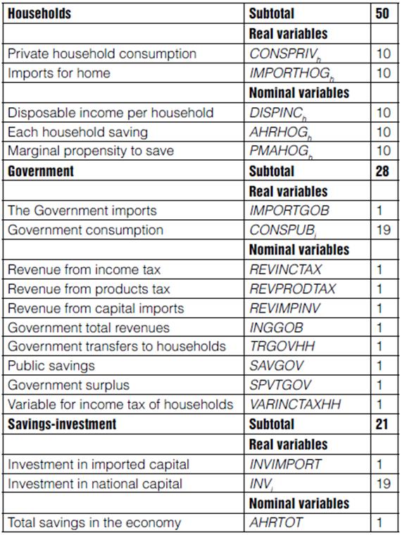
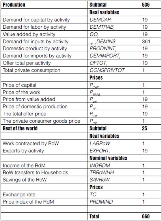
This section describes the mathematical model. The equations of the model are specified. Table 12 describes the parameters and Table 13 the variables.
The AGEM-Mx08 Equations
Following the SAM ordering, we start to specify the equations we start with Households, using 4 blocks of behavioral equations. Disposable income of each household is equal to its capital and labor income (putting together effective social benefits and other social benefits for the sake of simplicity), from which households pay income tax; then, transfers from Government and from the RoW complete their income. In what follows, please refer to Tables 12 and 13 for a detailed explanation of parameters and variables.
 Out from their disposable income, households dedicate a proportion to save (Marginal Propensity to Save):

And the rest is allocated to goods imported directly from the RoW, and goods from the domestic economy. Households have Cobb-Douglas preferences on imports and a composite good for private consumption. This composite good pays the tax on products (mainly VAT):


We continue with Government, for which we define four variables for income and four for expenditures. The public fundraising total is the sum of revenues by Income Tax (Households and Capital), Taxes on products and production (Households and Activities), and Taxes on the import of capital goods:

Total income tax revenue equals income tax from households plus that from firms:
Revenue from taxes on products and production is the sum of taxes paid by Households, plus taxes on products and other taxes on production paid for Activities. We impute the taxes paid by the activities, including those of imports, to domestic production:

And revenues from imports of capital goods:

Regarding Government outlays, we assume that the policy is to allocate a fixed proportion of total collection to each element of public expenditure:
Now consider the savings-investment account. Total savings of the economy equal the sum of savings by each institution:

The economy assigns a fixed fraction of total savings to import capital goods; the tax is included in the price of imported capital goods:

The block of equations corresponding to the macroeconomic closure that equals total savings to total investment is placed below, in the last section of equations, devoted to macro-closures.
We now turn to model the production of goods and services, assuming it is carried out in three stages: 1) production factors are combined to generate Value Added (VA), 2) total supply inputs are added to generate domestic production, and 3) imported inputs are added to domestic production to generate the total supply.
Consider the first nesting, generation of value added (VA), where there are two blocks of variables for the demands of factors and a block of prices for the VA generated by each Activity. Assuming a function of Cobb-Douglas production with constant returns to scale, and minimization of costs, we obtain the optimum demands:
And assuming perfect competition (price equals average cost):

Similarly, for domestic production (DOMPRODN) there are three blocks of variables, one for the demand of VA, one for inputs, and the third for prices. Considering a Leontief combination, optimum demands are:
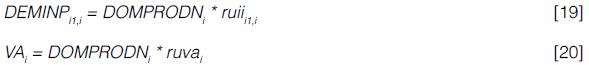
And from the assumption of perfect competition:

Now, with respect to production of Total Supply (SUPTOT) we have three blocks of variables, one for domestic production demand, another one for imported inputs demand, and the third for prices. Also assuming a Cobb-Douglas production function, with constant returns to scale, from the problem of cost minimization, optimal demands are:
And from the assumption of perfect competition:

The block of variables of total supply is determined by the equilibrium condition of market clearing. We also place this block at the end, in the macro-closures section.
Total private consumption equals the sum of Households demands:

Then, we define the price of the private consumption composite good, also given by the condition that unit price be equal to the average unit cost:

Finally, there is the Rest of the World, whose equations are:
RoW revenues (at RoW prices):
RoW expenses (at RoW prices):


With respect to the RoW, we adopt the small country assumption, which implies that all the prices of the RoW will remain constant and equal to 1.
As for macroeconomic closures, the first two equations to close the model, are given by the equilibrium in factor markets:
Then we have the basic closure for Savings-Investment: Marginal Propensity to Save (MPS) fixed, Investment flexible:

Alternatively: fixed Investment, MPS flexible:
Finally, the closure for goods' markets is:

Analysis of Taxes on Hydrocarbons Extraction
According to the IOT-Mx08, taxes paid by sectors and total production are presented in Table 14. The Other taxes on production (OIP) are from Table 58 of the Accounts of Goods and Services (AG&S), where it is seen that Other taxes on the extraction of oil and gas (901 548.6) are 99.9% of the Other taxes on mining. The global tax rate in the penultimate column is calculated by dividing total taxes by production at basic prices. In the last column the tax rate by sector is calculated, with data obtained for the MCS-Mx08, dividing total taxes by domestic production net of taxes.
Table 14 Taxes on Productive Sectors
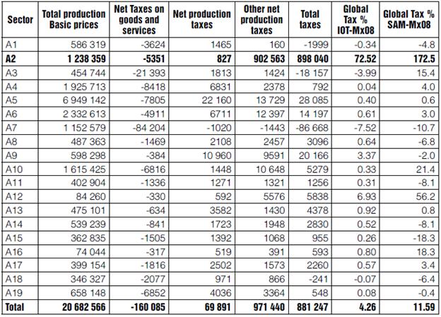
Source: Compilation with data of the MIP-Mx08 and CByS (INEGI, 2010a).
According to SAM's data in the last column, Mining pays a global tax of 172.5%; and the average tax rate paid by all sectors amounts to 11.59%. The simulation we implement decreases Mining taxes from 172.5% down to the average tax of 11.59% assuming that, after the reform of 2013, hydrocarbons extraction would pay a tax close to that average.
Table 15 shows the income tax rate paid by households according to the SAM-Mx08, which goes from 1.1% on the poorest decile, to 6.2% on the richest one.
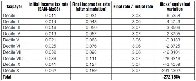
The simulation we implement reduces the total tax rate paid by Mining (hydrocarbons extraction) down to the average level of 11.59%, compensating with a uniform increase to income tax paid by households, so that (nominal) global revenue remains at the same level.
Macroeconomic closure
Since effects on households' wellbeing are a major concern for this research, we use Hick's Equivalent Variation (HEV) to evaluate changes in monetary terms. In order to compute a sensible HEV we set the following macro-closures combination: a) fixed real investment with flexible households savings (MPS h ), to prevent fluctuations in investment from biasing the HEV; b) fixed total government revenues and flexible Income Tax on Households, so that Government maintains the level of spending, and the welfare of households is not affected by the change in the consumption of public goods; c) by the same token, for the RoW we specify fixed income (and hence fixed RoW savings), and flexible exchange rate.
Simulation results
The implementation of the described simulation shows that reducing the tax on Mining (extraction of hydrocarbons), from 172.5 to 11.59%, to keep constant total government revenue would triple the income tax paid by households. The resulting simulation rates are also in Table 15; the penultimate column results from dividing the final rate by the initial.
In the last column are Hicks' Equivalent Variations, which show that lower income deciles are benefited, while from decile V on households begin to have a negative HEV due to the progressive income tax; if we sum up all ten of them, we obtain a negative total of (-272.1584) which accounts for total welfare loss in monetary terms. This negative effect obeys primarily to the fact that, with this reform, households have to pay for public services that were financed with taxes on Mining and, although a positive effect is observed through a fall in prices, this is much smaller and surpassed by far by the negative effect.
Table 16 contains the prices resulting from the simulation, which decrease more or less depending on the degree of integration of each sector with Mining. The price of labor increases slightly (0.1%) and final consumption prices decrease by 3.5%.
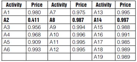
By construction, the AGEM-Mx08 is a model of perfect competition (although in this case Pemex is a monopoly; the small country assumption implies that it can't modify international oil prices). Therefore, price formation occurs from costs and taxes; hence, to lower taxes in Mining reduces its prices, which in turn lowers prices in other sectors, which would improve the competitiveness of the Mexican economy.
According to the simulation, the mining sector prices decrease by 59% (but as we said, international markets could prevent oil prices from decreasing). Consequently, prices in other sectors decrease from 0.3% in activity 14 up to 9.1% in activity 5 (which uses more imputs from the mining sector).
Conclusions
The first goal of this research was to build a Social Accounting Matrix of Mexico for 2008 (SAM-Mx08), fully transparent and documented, which we consider to be a relevant achievement in itself, providing a complete view of the Mexican economy and enabling the application of a wide range of analytical methods (Breisinger, Marcelle & Thurlow, 2010).
We believe that transparency is an essential criterion, which will allow results from investigations carried out with the SAM database to be replicated by other researchers and to be sufficiently discussed to arrive to solid and useful conclusions. Moreover, the SAM can be corrected and/or modified to do further studies. In addition, the SAM can be immediately broken down to the next level of the North American Industry Classification System (NAICS) with 79 subsectors (INEGI, 2013b), and even to the level of 262 branches, which enables a more detailed and comprehensive understanding of the economy.
To build the SAM, we assumed some simplifications in order to reconcile inconsistencies between the IOIT and the National Accounts; while it is commendable that INEGI has restarted the five-year development of the IOT for Mexico, it is also desirable that data in future editions be properly reconciled, so that the information is reliable and consistent for the public and private decision-making, and to enable scholars to perform deeper and more comprehensive economic investigations. INEGI might also consider the elaboration of a comprehensive SAM at least at the national level, and generate the necessary data so that researchers can build OITs and SAMs at the state and other regional levels.
The second objective was to develop a robust and parsimonious Applied General Equilibrium Model of Mexico for 2008 (AGEM-Mx08) based on the SAM-Mx08. In this we also believe that transparency is essential, because only the replication of results by other researchers and reasoned discussion will lead to valid and useful results. Therefore, both the SAM and the GAMS code for the AGEM will be provided by the author upon request.
In the same way, the AGEM-Mx08 may also be modified to apply it to the study of other problems, since we believe that its parsimony and robustness allow it to serve as a base or starting point for more complex models and more sophisticated simulations. The range of possibilities is wide: analysis of reform of VAT, effects of changes in public spending policies, evaluation of programs to alleviate poverty, international trade, etc.
The third objective was to apply the AGEM to a problem of high current interest in the Mexican economy and public finances: taxes on the extraction of hydrocarbons. This as accomplished with a simulation that is a first approach to a complex problem and that requires additional developments, for instance: a) A more elaborated specification of the functions of production and price formation, particularly in the extraction of hydrocarbons; b) Use of alternative closures and discussion of its implications on the results; and c) a more detailed assessment of impact on finances and spending, and their consequences for the welfare of households.
Results from the simulation we implemented indicate that even though low-income households would benefit slightly when reducing the taxes paid by the extraction of hydrocarbons and compensating with an equivalent increase in Income Taxes, households with higher incomes would have to absorb the financing of public expenditure, incurring in a high cost.

