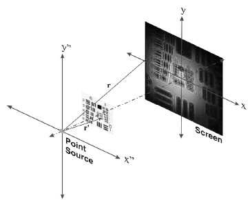
Figure 1. DIHM general schematic diagram
MODELACIÓN Y RECONSTRUCCIÓN DE HOLOGRAMAS TIPO GABOR
GABRIEL J. LORA
Escuela de Física, Universidad Nacional de Colombia Sede Medellín, gjloraj@gmail.com
NATALIA MUNERA
Escuela de Física, Universidad Nacional de Colombia Sede Medellín, nmunerao@gmail.com
JORGE GARCIA-SUCERQUIA
Universidad Nacional de Colombia Sede Medellín, jigarcia@unal.edu.co
]]> Received for review January 21th, 2010, accepted October 11th, 2010, final version October, 19th, 2010
ABSTRACT: The processes of modelling and reconstruction of holograms are based on the calculation of the diffraction integral either on its kirchhoff-fresnel or rayleight-sommerfeld formulation. Numerically, such an integral can be evaluated via different approaches: the convolution theorem, angular spectrum, and fresnel transform, among others. In this paper, the modelling of gabor-type in-line holograms of opaque particles of different diameters is presented. Those holograms are thereafter reconstructed by the numerical evaluation of the diffraction process that a spherical wavefront undergoes when it illuminates the hologram. The modelling-reconstruction process is employed for studying the performance of digital in-line holographic microscopy while the concentration of a simulated monodispersed monolayer is varied.
KEYWORDS: Digital in-line holographic microscopy, diffraction, hologram reconstruction, microscopy.
RESUMEN: Los procesos de modelación y reconstrucción de hologramas se soportan en el cálculo de la integral de difracción en su formulación de kirchhoff-fresnel o rayleight-sommerfeld. Dicha integral puede ser evaluada numéricamente por medio de diferentes formalismos: teorema de convolución, espectro angular y transformada de fresnel, entre otras. En este trabajo se presenta la modelación de hologramas en línea tipo gabor de partículas opacas de diferentes diámetros. Estos hologramas son reconstruidos por el cálculo numérico de la difracción que sufre una onda esférica cuando ilumina el holograma. El proceso de modelación-reconstrucción se utiliza para estudiar el desempeño de la microscopia holográfica digital en línea en función del cambio en la concentración de monocapas mono-dispersadas de esferas opacas.
PALABRAS CLAVES: Holografía digital en línea, difracción, reconstrucción de hologramas, microscopía.
1. INTRODUCTION
The possibility of having 3D representation objects that only exist in a designer’s mind, the ability of measuring cellular phenomena occurring at nanometre scales, among many other fascinating technological developments, partially rely on the fast growth of computing systems. Particularly, the two examples presented above are a reality, because it is now possible to compute light propagation in very efficient ways, i.e. it is now feasible to numerically compute diffraction processes via very efficient and robust algorithms. Today transmittance functions that after being correctly illuminated reproduce 3D images can be computed with such realism that the brain cannot distinguish them from a real object [1].
This technique is known as computer generated holography (CGH) and it was born with the work developed by Lohmann [2]. In another different but related application, from an apparently messy intensity recording it is possible to decode nanometre information that helps one to get a better understanding of cellular behaviour and that drives the development of new medicines; this technological development is named digital holography (DH) and it has its origin in Goodman’s work [3]. By this breakthrough, the feasibility of retrieving the complex wavefield from a digitally recorded interferogram was shown for the first time.
]]> Both CGH as well DH have extensive fields of application in technology and science. Perhaps CGH will lead to holographic cinema in the near future, while the most fascinating application of DH is digital holographic microscopy (DHM).DHM is a microscopy technique that cleverly merges the already amazing properties of holography with the power and versatility of the digital world. In DHM, it is possible to recover information from phenomena happening at scale ranges even below the illumination wavelength. Information coming from those ranges it is only recorded on the phase of a propagating wave. DHM, as the first microscopy technique that allows for quantitative retrieving of phase information, has brought this new possibility into play.
Mainly two different approaches to DHM are recognized, one that uses lenses and regularly plane waves, and the other which uses spherical waves and no lenses. Due to the limited spatial resolution of the commercially available digital cameras, to record enough information from the holograms one needs to enlarge them before their recording. While it is the role of the lenses in plane wave DHM, in DHM with spherical waves, the simple propagation of the wave enlarges the hologram before its recoding.
The newest approach to DHM is named digital in line holographic microscopy (DIHM) [4] and is highlighted for its simplicity and robustness. Figure 1 illustrates a typical DIHM setup. In DIHM, a point source illuminates a sample located at the plane denoted by vector. The interference pattern produced by the portions of the spherical wave disturbed and not disturbed by the sample is digitally registered in a CCD or CMOS camera. This record, called a digital hologram, is stored in the memory of a computer for its further analysis. The step that leads to a digital hologram is known as the recording process.
Figure 1. DIHM general schematic diagram
Once in the memory of a computer, the digital hologram passes through minimum image processing and a further process that leads to recovering the object information. This latter process is known as the digital hologram reconstruction and is totally numerically performed. In DIHM, the reconstruction stage of the hologram is carried out through the numerical calculation of the diffraction process that a spherical wave suffers as it illuminates the digital hologram. In the same way that it happens in optical holography, two reconstructed images are obtained, virtual and real images, which constitute what are called twin images [4,5]. Although it has simplicity in hardware and software, DIHM can achieve lateral resolution of the order of the illumination wavelength [4].
In order to study the features and possibilities of DIHM, it becomes very useful to model the recording and reconstruction processes, in a wholly numerical approach. Both steps involved in DIHM are described by the diffraction that a spherical wavefront undergoes as it illuminates a sample/digital hologram in the recording/reconstruction process. Therefore, in order to fully and numerically model the DIHM, one needs to efficiently compute the diffraction phenomena in either Kirchhoff-Fresnel or Rayleight-Sommerfeld formalism [5]. In turn, the development of discrete tools for fully numerical modelling of DIHM is presented in this work. By definition, the digital hologram is numerically reconstructed. However it is necessary to develop appropriated algorithms for computing the diffraction process that the spherical wave undergoes on the sample, which gives rise to the digital hologram. The numerical model of DIHM is applied to a first endeavour for studying the limits on the sample concentration that can be analysed with DIHM.
2. CALCULATION OF THE DIFFRACTION INTEGRAL IN DIHM
]]> The diffraction phenomena that take place in DIHM, for recording as well for hologram reconstruction, are correctly described by the scalar approximation to the diffraction theory [5, 6]. In this approximation, the polarization effects of electromagnetic waves are neglected and the wave equation becomes the Helmholtz equation. Its solution for free space expresses the optical field on an observation point P through the Fresnel–Kirchhoff diffraction integral [5,6] (1)
(1)
In equation (1)  is the wavelength,
  is the wave number,
  is the optical field amplitude at the
  plane,
  and
and  , as illustrated in Figure 2. Equation (1) has an analytical solution in very restrictive cases, mainly with just academic interest. For most of the practical situations, the optical field on the observation plane is found via numerical and/or approximated forms. For modelling DIHM, the evaluation of the diffraction phenomena in both of its stages, recording and reconstruction, should be carried out through numerical methods compatible with the typical experimental setups. Some experimental conditions of DIHM which constitute a challenge for numerical evaluation of equation (1) are: i) numerical apertures higher than 0.3 in connection with the specifications of the devices available in the market for digital recording, and ii) point source-sample distance of the order of 1500µm. The need for evaluating systems with numerical apertures higher than 0.3 resides in the fact that lateral resolution of DIHM, i.e., the minimum distance
  to which the system differentiates two objects, is controlled by:
 (2)
(2)
with NA numerical aperture of system. Therefore, with NA = 0.3 the maximum feasible resolution is of the order of 900nm for a typical  nm. To achieve this resolution with the cameras available in the market of 1024x1024 square pixels of 6μm each side, indicates a maximum distance of 9.8mm from the point source to the camera [7]. The maximum distance point source-sample in order to achieve such a resolution is 1 mm [7].
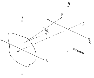
Figure 2. Coordinate system used to evaluate the equation (1)
In summary, this set of conditions imposes challenges in the modelling processes since, as it will be shown, many algorithms simply do not work or the involved phases in the process are not correctly sampled. Three of the different methods that are found in the literature for the numerical calculation of the diffraction equation (1) are briefly discussed in the following: angular spectrum, convolution theorem, and Fresnel approximation.
2.1. Angular spectrum
As the optical field is considered to be composed by plane waves propagating in all directions, the field can be written as [5]:
 (3)
(3) with  the angular spectrum of the optical field at
  plane.
 is given by the angular spectrum on entrance plane
  once a
  distance is propagated:
 . (4)
. (4)
In equations (3) and (4)  are the spatial frequencies along the
  coordinates, respectively. Any combination of spatial frequencies that lay outside of the circle defined by
  gives rise to evanescent waves; for DIHM such a regime is avoided. The decomposition of the entrance optical field in terms of plane waves indicates that the angular spectra correspond to the Fourier transforms of the fields. In this way the angular spectrum in the entrance plane
  is:
is:
 . (5)
. (5)
Because the Fourier transform operator  has a simple and optimized computational implementation, it is convenient to write down the amplitude of the optical field in a plane
  away from the aperture as:
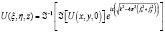 . (6)
. (6)
The Fourier Transform operator  is implemented through fast Fourier transform (FFT), which permits the rapid calculation of the amplitude of the optical field.
2.2. Convolution
The diffraction phenomenon can be cast into a linear process [5] if in equation (1),  and it is rewritten as:
 . (7)
. (7) In equation (7)  is the transfer function for the free space, and it is defined as:
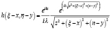 . (8)
. (8)
Equation (7) is recognized to be a convolution between  and
and  , therefore it can be calculated through the convolution theorem [5]:
 . (9)
. (9)
Because of its representation in terms of  operator, equation (9) can also be evaluated through FFT. As much the angular spectrum as well as the convolution method allow for computing the diffraction integral without dramatic approximations. This fact makes these methodologies quite attractive for modelling DIHM experiments.
2.3. Fresnel approximation
The simplest method for numerical calculation of the diffraction integral is the Fresnel approximation. This scheme can be employed when the considered distances in the experiment are correctly expressed through a parabolic approximation. It has validity when  , since for this regime the distance
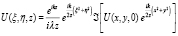
  is well represented by the two first terms of its series expansion [5]. Once such terms are introduced in the diffraction integral (1) and it is rewritten in terms of Fourier operators, the optical field at
  plane is given by:
 (10)
(10)
The optical field on the  plane can be calculated as the FFT of the optical field on
  plane,
  , modified by the Fresnel phase
  . The result from this transform is multiplied by the phase terms in front the operand
  , as is shown in equation (10).
The application ranges for the three methodologies here exposed are summarized in Table 1 [8]; without lack of generality, only one dimension has been accounted for. In Table 1, it is considered that the optical field is sampled by M pixels, each one of  width. In these terms, the numerical aperture of system is given by:
 (11)
(11)
therefore, if a camera with M = 1024 and = 6um is considered, to obtain NA = 0.3, the z distance, the point source-camera distance should be equal or smaller than 9.8mm. According to Table 1, for a typical λ of 500nm the Fresnel approximation imposes z > 73.7mm, which excludes this approach for calculating in DIHM. The utilization of the angular spectrum or the convolution approximation is identical in terms of the minimum distance imposed by the conditions of Table 1; according to this Table z ≤ 73.7 mm, which enables both approaches for calculating in DIHM. From this point of view, the results reached with one or another methodology are completely equivalent. For validating this analysis in Figure 3, a modelling example of DIHM holograms is shown.
Table 1. Application range of the methods for calculating the diffraction integral
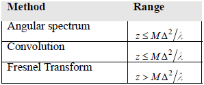
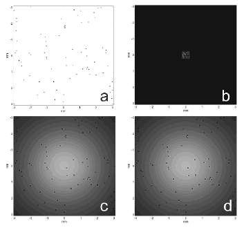
Figure 3. In-line hologram DIHM-type modelling. a Transmittance function located at a distance of 3mm from the point source. Results of the diffraction evaluation as the transmittance function is illuminated by a spherical wave, b Fresnel approximation, c spectrum angular, and d Convolution
Figure 3 shows the results of in-line holograms DIHM-type modelling. In panel a, the transmittance function of the sample is shown; it is generated by considering 13 identical particles of a 20µm radius; the transmittance is placed on a plane 3mm away from the point source. The specifications of the hologram plane equal those of the camera CCD: 1024 pixels along each direction with individual pixels of 6x6um2. In panel b the modelled in-line hologram is presented through the Fresnel approximation. Due to the limited area of the hologram plane that is used, from this recording it is not possible to recover the transmittance function. Furthermore, this recording does not resemble the sort of holograms that are recorded in a DIHM experiment. Panels c and d show the DIHM holograms modelled with angular spectrum and convolution approaches, respectively. In both of the cases, the full field of view of the hologram is employed and from these kinds of intensities it is possible to retrieve the information of the transmittance function. These modelled holograms resemble the intensity that is recorded in an equivalent DIHM experiment. Because of the similitude of the modelled in-line holograms with these two approaches, it is valid to employ any of them. If the contrary is not stated, the convolution methodology is employed for modelling the in-line holograms shown below.
]]>3. DIHM NUMERICAL MODELLING
As is done in DIHM experiments, the modelling process is carried out in two stages: the recording and the reconstruction steps.
In the recording stage, a spherical wavefront illuminates a sample located at a distance  from the point source; numerically this process is carried out by means of considering the exact analytical expression of the spherical wavefront on the sample plane. For the whole modelling process the point source is accounted as being the coordinate origin. The sample is generated by randomly placing opaque particles of a chosen radius; a hexagonal layout on the sample plane guarantees that neighbour particles are packed following hexagonal packing as is shown in Figure 4. On the sample plane, a pixel-wise product between the spherical wavefront and the transmittance function leads to the complex amplitude being propagated towards the CCD plane. Such a complex amplitude constitutes the
  input for equation (9). Via this same equation
  a
a  distance is propagated for reaching the hologram plane, where the CCD camera is located. The recorded hologram corresponds to the square modulus of the complex output from equation (9).
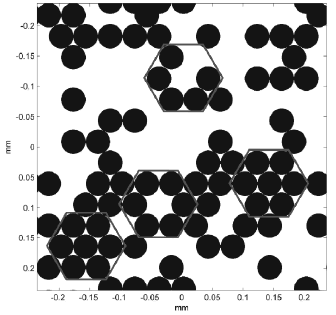
Figure 4. Hexagonal packed monolayer of opaque microspheres used as transmittance function. The red hexagons show the pack type
In the reconstruction stage, the intensity distribution produced by a point source placed at an  distance from the hologram plane, is pixel-wise subtracted from the modelled hologram. This new intensity distribution is known as the contrast hologram [4]. Because the information of the spherical wavefront without any perturbation from the object is subtracted from the hologram, this operation gets rid of any noise or oddness of the illumination. The contrast hologram is then propagated an
  distance to get an intensity distribution that represents the sample. In order to attempt this reconstruction process, different approaches can be found in the literature. The most widely used is the Kirchhoff-Helmholtz transform which is implemented via a scalable convolution [4].
Replicas of the original Gabor’s holograms have been reconstructed by using a different version of the convolution approach [9]. Molony et al. [10] have proposed a reconstruction method based on Fresnel’s transform of the recorded or modelled hologram; angular spectrum and direct calculation of Fresnel’s integral are evaluated in order to test their applicability in DIHM.
In Figure 5, the whole modelling process is shown. Panel a shows the sample transmittance function; 500 particles of 20µm radius have been randomly placed on the sample plane. The modelled Gabor-type hologram is presented in panel b, and the contrast hologram and the corresponding reconstruction are shown in panels c and d, respectively. Both stages of the DIHM modelling, recording and reconstruction, have been carried out by using the convolution methodology.
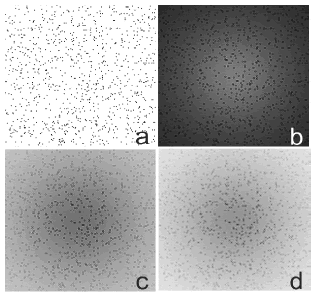 ]]>
Figure 5. Complete DIHM modelling process. Panel a shows the sample transmittance function. Panel b presents the Gabor-type hologram. The contrast hologram and its reconstruction are shown in panel c and d, respectively. All the images are 6x6mm2
]]>
Figure 5. Complete DIHM modelling process. Panel a shows the sample transmittance function. Panel b presents the Gabor-type hologram. The contrast hologram and its reconstruction are shown in panel c and d, respectively. All the images are 6x6mm2
Modelling tools are of great utility for studying the limit performance of a technique under well controlled situations. Particularly in the case of DIHM, it is quite interesting to find out the limit of the sample concentration that can be evaluated through this microscopy methodology; this point is addressed in the following section.
3.1. Effect of particle density on the DIHM performance
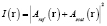
As illustrated in Figure 1, the recorded intensity of the CCD or CMOS camera on the hologram plane of a DIHM experiment, is given by the
square modulus of the amplitude superposition of the portion of the spherical wave that is scattered by the object  and that portion that does not
  :
:
 . (12)
This equation represents the Gabor-type hologram and the contrast hologram is then obtained by the pixel-wise subtraction between equation (12) and the intensity provided by the point source over the hologram plane  , explicitly leading to:
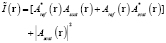 (13)
(13)
In equation (13), the terms between the square brackets represent the twin images of holography [4,5]. The remaining term signifies the intensity scattered by the object. Since the original proposal of holography by D. Gabor, this term has been recognized as negligible with respect to the others that constitute the hologram [11]. This affirmation is valid when transparent objects are considered or when the number of the opaque objects that scatter the incoming spherical wave is very "low" per area unit. Through modelling the complete DIHM of Gabor-type holograms of monodispersed monolayers of microspheres, it is possible to establish a quantitative limit that dictates the number of particles per area unit that makes Gabor’s approximation valid. Since DIHM is based on Gabor’s approximation, this limit allows for establishing the ranges of the applicability of this microscopy methodology.
The performance of DIHM, can be evaluated by comparing the sample transmittance function and the reconstructed hologram. The procedure adopted for this evaluation has been to considering the point-wise subtraction between the reconstructed intensity and the sample transmittance function. Then the sum over all the pixels of this subtraction is accounted as being the control criterion. The value of this criterion has been plotted versus the number of particles of the sample, with the results shown in Figure 6.
]]>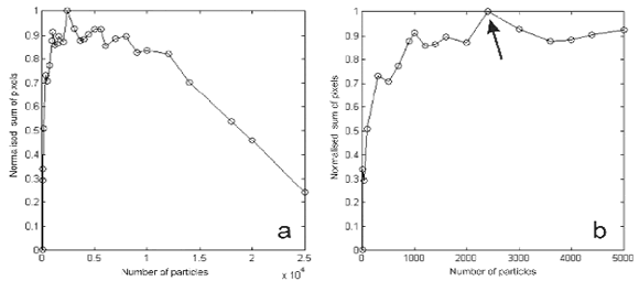
In panel a, the behaviour of the criterion control for a number of particles between 1 and 25,000 is present; the same it is shown in panel b, between 1 and 5,000 particles. From the behaviour of these curves, it can be concluded that for a number of particles lower than 500, there is great similarity between the sample transmittance function and the corresponding reconstructed intensity; the meaning of this result is that DIHM performs quite well in this range. From that number of 500 particles, the value of the control criterion increases and reaches a maximum value of about 2,400 particles, indicated by the arrow in panel b. As the reconstructed intensities and the sample transmittance functions are visually compared for the number of particles below and above that limit number, it is found that for this particular DIHM modelled experiment, 2,400 is the order of the maximum number of particles that can be correctly imaged with this microscopy methodology
To generalize the former result of the number of particles that can be correctly imaged with DIHM, the number of particles per area unit has been computed. The sample plane has been placed at  , and the hologram recorded on a camera of 6.1x6.1 mm2 that subtends
  ; therefore Gabor’s approximation is valid for an order of 500particles/mm2 for individual particles with a 20µm radius; this result is equivalent to saying that 62% of the incoming illumination is blocked out by the sample. Therefore, it can be proposed that Gabor’s approximation about the negligibility of the amplitude of the scattered wavefront is valid if at least 38% of the incoming spherical wavefront passes through the sample without being perturbed.
4. CONCLUSIONS
In summary, algorithms for modelling in-line holograms, of the digital in-line holographic microscopy (DIHM)-type, have been developed. Due to the operation conditions of DIHM, it has been found that the Fresnel approximation does not correctly describe the diffraction processes that take place in DIHM. Because of this reason, the convolution formalism has been utilized for modelling the in-line Gabor-type holograms and for their reconstruction.
The tools developed here have been utilized to validate the range of operation of DIHM in terms of particle concentration. It has been found that at least 38% of the incoming spherical wave must travel directly towards the detector for DIMH to work.
The similarities between the sample transmittance function and the reconstructed intensity have been accounted for a proposed control criterion. This criterion takes the sum of the input pixels of the resulting matrix from the pixel-wise subtraction between the sample transmittance function and the reconstructed image. Different merit functions that could make an estimate of the differences between the proposed sample and the reconstructed image from the modelled hologram should be looked for.
]]> ACKNOWLEDGEMENTS
The authors thank DIME (Universidad Nacional de Colombia, Sede Medellín) and DINAIN (Dirección Nacional de Investigacion UNAL) for the economic support. This work was partially supported by the Universidad Nacional de Colombia through the Bicentenario program under Grant 90201022.
REFERENCES
[1] http://www.zebraimaging.com/ [ Links ]
[2] LOHMANN, W. AND PARIS, D., "Binary Fraunhofer holograms generated by computer," Appl. Opt. 6, 1739-1748, 1967. [ Links ]
[3] GOODMAN, J. AND LAWRENCE, R, Digital image formation from electronically detected holograms, App. Phys. Lett. 11, 77-79, 1967. [ Links ]
[4] GARCIA-SUCERQUIA, J., XU, W., JERICHO, S., KLAGES, P., JERICHO, M. and KREUZER, H., Digital In-line Holography Microscopy, Appl. Opt. 45, 836-850, 2006. [ Links ]
[5] GOODMAN, J., Introduction to Fourier Optics, McGraw- Hill, New York, 1968. [ Links ]
[6] BORN, M. AND WOLF, E., Principles of Optics, Pergamon Press, Oxford, 1993. [ Links ]
[7] JERICHO, S., GARCIA-SUCERQUIA, J., XU, W., JERICHO, M. and KREUZER, H., Submersible Digital In-line Holographic Microscope, Rev. Sci. Inst. 77, 043706,1-10, 2006. [ Links ]
[8] SYPEK, M., PROKOPOWICZ, C. and GORECKI, M., Image multiplying and high-frequency oscillations effects in the Fresnel region light propagation simulation, Opt. Eng. 42, 3158-3164, 2003. [ Links ]
[9] REPETTO, L., PELLISTRI, F., PIANO, E. and PONTIGGIA, C., Gabor's hologram in a modern perspective, Am. J. Phys. 72, 964-967, 2004. [ Links ]
[10] MOLONY, K., HENNELLY, B., KELLY, D. and NAUGHTON, T., Reconstruction algorithms applied to in-line Gabor digital holographic microscopy, Opt. Comm, 283, 903-909, 2010. [ Links ]
[11] GABOR, D., Microscopy by reconstructed wave-fronts, Proc. Roy. Soc. London A. 197, 454-487, 1949. [ Links ] ]]>