, we estimated, in joint form, the parameters of the life stress model and one shape parameter . These were then used to extrapolate the conclusions to the operational level. However, these conclusions are biased because in the experiment design (DOE) used, each combination of the variables presents its own Weibull family . Thus the estimated is not representative. On the other hand, since is determined by the variance of the logarithm of the lifetime data , the response variance and the correlation coefficient , which increases when variables are added to the analysis, is always overestimated. In this paper, the problem is statistically addressed and based on the Weibull families a vector is estimated and used to determine the parameters of . Finally, based on the variance of each level, the variance of the operational level is estimated and used to determine the operational shape parameter . The efficiency of the proposed method is shown by numerical applications and by comparing its results with those of the maximum likelihood method (ML).]]>
, estimamos en forma conjunta los parámetros del modelo de relación vida esfuerzo y un parámetro de forma . Después estos parámetros son utilizados para extrapolar las conclusiones al nivel operacional. Como sea, estas conclusiones están sesgadas debido a que dentro del diseño de experimentos (DOE) utilizado, cada combinación de las variables presenta su propia familia Weibull . De esa forma la estimada no es representativa. Por otro lado, dado que está determinada por la varianza del logaritmo de los tiempos de vida , por la varianza de la respuesta y por el coeficiente de correlación , el cual crece cuando se agregan variables al análisis, es siempre sobre estimada. En éste artículo, el problema es estadísticamente identificado y basado sobre las familias Weibull un vector es estimado y utilizado para determinar los parámetros de . Finalmente, basado en la varianza de cada nivel, la varianza del nivel operacional es estimada y utilizada para determinar el parámetro de forma del nivel operacional. La eficiencia del método propuesto es mostrada a través de aplicaciones numéricas y por la comparación de sus resultados con los del método de máxima verosimilitud (ML).]]>
Weibull accelerated life testing analysis with several variables using multiple linear regression
Análisis de pruebas de vida acelerada Weibull con varias variables utilizando regresión lineal múltiple
Manuel R. Piña-Monarrez a, Carlos A. Ávila-Chávez b & Carlos D. Márquez-Luévano c
a Industrial and Manufacturing department of the IIT Institute, Universidad Autónoma de Ciudad Juárez, Chihuahua , México. manuel.pina@uacj.mx b Industrial and manufacturing deparment of the IIT Institute, Universidad Autónoma de Ciudad Juárez, Chihuahua , México. carlos.avila@uacj.mx c Reliability Engineering Department at Stoneridge Electronics North America. carlos.marquez@stoneridge.com
]]>
Received: May 16th, 2014. Received in revised form: February 24th, 2015. Accepted: March 04th, 2015
Abstract In Weibull accelerated life test analysis (ALT) with two or more variables , we estimated, in joint form, the parameters of the life stress model and one shape parameter . These were then used to extrapolate the conclusions to the operational level. However, these conclusions are biased because in the experiment design (DOE) used, each combination of the variables presents its own Weibull family . Thus the estimated is not representative. On the other hand, since is determined by the variance of the logarithm of the lifetime data , the response variance and the correlation coefficient , which increases when variables are added to the analysis, is always overestimated. In this paper, the problem is statistically addressed and based on the Weibull families a vector is estimated and used to determine the parameters of . Finally, based on the variance of each level, the variance of the operational level is estimated and used to determine the operational shape parameter . The efficiency of the proposed method is shown by numerical applications and by comparing its results with those of the maximum likelihood method (ML).
Keywords: ALT analysis; Weibull analysis; multiple linear regression; experiment design.
Resumen En el análisis de pruebas de vida acelerada Weibull con dos o más variables aceleradas , estimamos en forma conjunta los parámetros del modelo de relación vida esfuerzo y un parámetro de forma . Después estos parámetros son utilizados para extrapolar las conclusiones al nivel operacional. Como sea, estas conclusiones están sesgadas debido a que dentro del diseño de experimentos (DOE) utilizado, cada combinación de las variables presenta su propia familia Weibull . De esa forma la estimada no es representativa. Por otro lado, dado que está determinada por la varianza del logaritmo de los tiempos de vida , por la varianza de la respuesta y por el coeficiente de correlación , el cual crece cuando se agregan variables al análisis, es siempre sobre estimada. En éste artículo, el problema es estadísticamente identificado y basado sobre las familias Weibull un vector es estimado y utilizado para determinar los parámetros de . Finalmente, basado en la varianza de cada nivel, la varianza del nivel operacional es estimada y utilizada para determinar el parámetro de forma del nivel operacional. La eficiencia del método propuesto es mostrada a través de aplicaciones numéricas y por la comparación de sus resultados con los del método de máxima verosimilitud (ML).
Palabras clave: ALT análisis; análisis Weibull; regresión lineal múltiple; diseño de experimentos.
]]>
1. Introduction
In Accelerated Life Testing analysis (ALT) with constant over time and interval-valued variables , the standard approach of the analysis consists in using higher levels of the stress variables and a life-stress model , the lifetime data are obtained as quickly as possible [6]. In this approach, the function , which relates the lifetime data to the stress variables, is parametrized as
Where is a vector of unknown parameters, and is a vector of specified functions with . Among the most common models of we have the generalized Eyring model, the temperature-humidity model (T-H), the temperature-non-thermal model, the proportional hazard model and the generalized log-linear model [9] and [13]. On the other hand, in ALT Weibull analysis no matter which model we use, all of them are used to estimate the scale parameter under different levels of the significant variables. For example if the (T-H) model is used, then in the Weibull probability density function (pdf) ([19] and [16] Chapter 1), given by
by replacing with the model the Weibull/(T-H) pdf is given by
Unfortunately, since in (3) only one shape parameter is estimated and used to represent all the level combinations of the variables, and because the maximum likelihood (ML) or multiple linear regression (MLR) methods perform the estimation as linear combination of with the coefficients of the vector is always overestimated. As a consequence, the related reliability is overestimated too. In order to show this problem, in section 2 the generalities of ALT analysis are given. Section 3 presents the problem statement. In section 4 the problem is statistically addressed. Section five details the proposed method and, finally, in section 6 the conclusions are presented.
2. Generalities of Weibull ALT analysis
]]>
In ALT analysis, the objective is to obtain life data as quickly as possible. Data are obtained by observing a set of n units functioning under various levels of the explanatory variables . These levels are chosen to be higher than the normal one. With these life data, we draw conclusions and then, the conclusions are extrapolated to the normal level. Models used to perform the extrapolation are known as life-stress models . Among the most common models we have the parametric accelerated failure time models (AFT) (e.g. Arrhenius model) [8], and the proportional hazard model (PH) (e.g. Weibull proportional hazard model) [5] and [1]. On the other hand, in the analysis, the lifetime data T is a nonnegative and absolute continuous random variable. Thus, the survival function is . And based on this, the corresponding probability density function is and the hazard rate function is . Additionally, it is important to note that in ALT, the effect that the covariates have over T, is modeled by , which as in (3) is included in . On the other hand, for constant over time and interval valued variables, the cumulative risk function is with parametrized as where and Z are as they were defined in (1), and represents the base risk when all the covariates are zero . For example, based on this formulation and on the physical principle of Sedyakin [1], pp. 20), the survival function for two different levels of the variables is related by . Implying that which in terms of mean that , and since the survival function does not depend on , then the random variable does not depend on X either. In particular observe that, since the expected value of is and its variance is , then its variation coefficient does not depend on either. Thus, for any two stress levels (or variables combination), the distribution is the same, implying that only the scale changes (see [1] sec. 2.3). Observe the fact that the scale only changing in the Weibull analysis implies that
On the other hand, R(t) under any two levels is related by where
and that it is called the acceleration factor. Finally, it is important to note that by setting or , and because and do not depend on , then as in (5), the variance of does not depend on either.
Despite of this, because in the estimation of the Weibull life-stress relationship as in (3), we estimate only one value as a linear combination of the variables , is always overestimated as in the following section.
3. Problem statement
Statement 1: Because in ALT failure time data is obtained by increasing the level of the variables , the variance of the logarithm of the lifetimes defined in (5) is diminished (the time to failure is shorted) and as a consequence, is overestimated.
Statement 2: In multivariate ALT analysis, when significant variables are added into , the relation between the logarithm of the scale parameter and tends to be one, thus the corresponding sum square error is diminished increasing , and as a consequence, is overestimated.
]]>
Considering these statements, firstly note that is intrinsically related to the strength characteristics of the product; thus, if the levels of the significant variables are selected in such that, for their higher effect combination, they do not generate a foolish failure mode (the effect of the level combinations is lower than the effect that reaches the destructive limits), must be constant, and its value must represent the variance of the strength characteristic which in the estimation processes with constant over time and interval-valued variables is not used (or measured). And second, we can observe that in the estimation process, the shape parameter is determined by the variance of the logarithm of the lifetime data , the response variance and the correlation coefficient , and that neither of them represent . Thus, due to the dependence of on , and , adding significant variables (increases R2) and/or overstressing their levels (diminishes ) always overestimates as in the following section.
4. Statistical analysis
Let us first show that is completely determined by , and . To see this, let us use the Weibull reliability function given by
Which in linear form is given by
Where , , , , and is the cumulative failure function of t given by . based on the median rank approach is estimated as [14].
For another possible approximation of F(t), see [3], [4] and [21]. On the other hand, observe from (7a) that is a critical parameter (see [10] and [16] sec. 2.3) and thus, the analysis depends on the accuracy by which it is estimated. Also, observe that (7b) is in function of the sample size n and that for the F(t) percentile is greater than 90% [2]. Regardless of this, note that represents the 0.367879 reliability percentile which corresponds to implying from (7a) that for center response Y
]]>
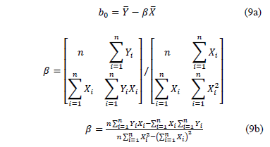
Thus, under multiple linear regression the coefficients of (7a) are estimated as
From (9b) observe that its denominator is the variance of the logarithm of the lifetime data defined in (5), which in terms of the covariates is given by.
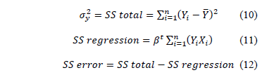
On the other hand, the goodness of fit of the polynomial given in (7a) is performed by the anova analysis where its sources of variation are
The goodness of fit index is given by
Finally from (9c), (10), (11) and (13), is given by
]]>
On the other hand, to see that increasing (or decreasing) affects as in Statement1, note from (8) that increasing (or decreasing) is equivalent to increasing (or decreasing) in (9b). That is to say, shortening the time in which the lifetime occurs, decreases their variance and thus, according to (14), is overestimated.
In the case of Statement 2, from (11) to (14), it is clear that although the levels of the variables are not stressed, by adding significant variables, since and , are fixed as in (5), then in (14) is increased, and as a consequence, is always overestimated.
5. Proposed Method
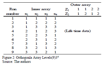
To see numerically that is overestimated as in section 4, first note that each combination of the variables, as in Fig. 1, presents its own Weibull family, and that data are gathered by using a replicated experiment design DOE as presented in Fig. 2 (see [15] and [20] Chapter 13).
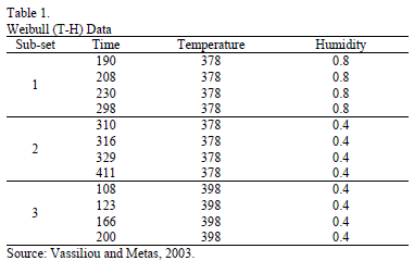
Second, to illustrate this, let us use the DOE data from Table 1, which corresponds to twelve electronic devices. Data were published by [17] p.11.
]]>
From these data, the Weibull/(T-H) parameters defined in (3), by using ML are , , and (the ALTA Pro software was used). In addition, observe that although in Table 1 there are three level combinations among the variables, which as a consequence lead to three Weibull families in this DOE, regardless of this, in the standard approach [eq. (3)], only one shape parameter was estimated.
Thus, it is not representative of the whole set of data. To see this, in Table 2, the scale and shape parameters , estimated by ML, and their associated reliability for t=150 are given.
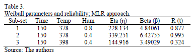
In order to compare the standard results of Table 2, with those found in the DOE, Table 3 presents the Weibull family and R(t) for each DOE combination, using (8) and (9b) with centered response (Y).
By comparing these results, we observe that the estimated in Table 2, in contrast to the estimated from Table 3, does not represent the expected 0.367879 percentile as defined in (8). And that does not represent the shape parameter of the levels found in the DOE. Thus the proposed method to avoid this issue, using MLR, is as in the following section.
5.1. Regression approach for statement 1.
In ALT with one interval valued and constant over time variables, as is the case of Weibull/Arrhenius, Weibull/Inverse power law and Weibull/Eyring, it is possible to estimate their parameters by applying (8), (9a) and (9b) by following the next steps.
Step 1. For each replicated level of the stress variable (We must have almost 4 replicates, although 10 are recommended), determine the corresponding and parameters by using (7a), (8), (9a) y (9b). (In this one variable approach, is generally constant). If is not constant, proceed as in section 5.2.
Step 2. Take the effect of the corresponding linear transformation (see next section) of the time/stress model defined in (1) as (e.g. in Arrhenius ) and the corresponding logarithm of the scale parameter of the i-th level of the variable estimated in step 1 as .
]]>
Step 3. Using (9a) and (9b), estimate by regression between the variables and defined in step 2, the parameters of the life/stress model .
Note: In the Eyring case, do not forget to subtract the logarithm of the reciprocal of the temperature from the logarithm of before you perform the regression.
Step 4. Using the regression parameters of estimated in step 3, estimate the logarithm of for the operational (or desired) level (see next section). Finally, form the Weibull family of the operational (or desired) level W() with the shape parameters estimated in step1 and the scale parameter estimated in this step. And with these Weibull parameters, determine the desired reliability indexes.
5.1.1 Let us exemplify the above methodology, through the Weibull/Arrhenius and Weibull/Eyring relationship, which are parametrized as in (1). In the case of Arrhenius, the infinitesimal characteristic (see [18]) is given by , thus the primitive (integral) of , is given by . Since shows the form in which the variable affects the time, in the Arrhenius model the effect is (see step 2 of section 5.1). Thus from (1) and (4), the Arrhenius model is given by: (for details see [1], Chapter 5).
In (15a), and are the parameters to be estimated, and T is the absolute temperature (Kelvin). The linear form of (15a) is given by
Using (15a) the Weibull/Arrhenius pdf is given by
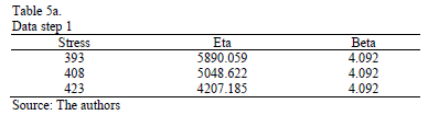
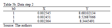
As a numerical application, consider the data in Table 4. Data were published by [17]. The Weibull parameters of step 1 are given in Table 5a. The effect for step 2, and are given in Table 5b.
]]>
The Weibull/Arrhenius parameters of step 3 using Minitab® and data of Table 5b, are and with . Finally, by using these parameters, the Weibull family mentioned in step 4, for a level of 323K is .
5.1.2 In the case of the Weibull/Eyring relationship the infinitesimal characteristic is given by , with primitive of , given by , thus . This formulation with is used in the Eyring model when the temperature is used. The Eyring model is given by:
In (17), and are parameters to be estimated and T is the absolute temperature. The linear relationship of (17) is
And the linear relationship used to estimate the parameters is given by
]]>
The Weibull/Eyring pdf using (17) is
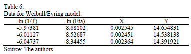
Using data of Table 4, the Weibull/Eyring parameters of step 3 using Minitab® with data of Table 6, are and with . By using these parameters the Weibull family mentioned in step 4, for a level of 323K is .
Finally, for the one variable case, when the shape parameter is not constant for all the stress levels proceed as in the multivariate case of the following section.
5.2. Regression approach for statement 2.
For the multivariate ALT analysis, as in Fig. 1, each covariate combination presents its own Weibull family. Thus, because in the standard ALT analysis, the estimated value does not represent the whole set of data, in MLR, we propose to estimate the Weibull/life/stress parameters through the following steps.
Step 1. For each replicated combination level of the stress variables (We must have almost 4 replicates; 10 is recommended; see comment below eq. (7b)), determine the corresponding Weibull family . This could be performed by ML, but MLR is recommended. (ML is a biased estimator and n is small).
Step 2. Take the effect of the corresponding linear transformation of the variables as the independent variables and the corresponding logarithm of the scale parameter of the i-th Weibull family of step1 as the dependent variable .
Step 3. Estimate the parameters of the life/stress model by regression between the set of variables and defined in step 2. If there are not enough degrees of freedom to perform the analysis, proceed as follows.
]]>
a) Estimate a vector by reordering (7a) as
Estimate the parameters of by performing a regression between and . In (20), is as in (7b), and and are the shape parameter and the logarithm of the lifetime data of the i-th Weibull families of step 1.
b) Based on (5) and on the fact that where is the sample variance of the lifetime data, form the logarithm vector
where is the variance of the i-th level defined in (9c) and n is the number of replicates of the i-th level of step1.
c) Take the inverse of the effect of the covariates of step 2, as the independent variables and as the response variable and perform a regression between and .
Observe that and are vectors for the complete DOE data (or families).
Step 4. Using the regression parameters of estimated in step 3-a), estimate the scale parameter for the operational level by applying (4). By using the regression parameters of step 3-b), estimate the value of of the operational level, and by applying (14), with of step 1 and a desired index, estimate the corresponding value. are the parameters of the Weibull family of the desired stress level and they could be used to determine any desired reliability index. Observe that the estimation of using (14) is robust (almost insensible) to the selected index.
As a numerical application consider the data in Table 7. Data were published in [17].
]]>
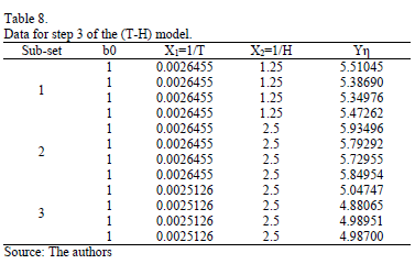
On the other hand, data of step 3 using (20) are given in Table 8. By using Minitab, the parameters of W(T-H) model by regression between and are , , and with . The parameters of the regression between and are , and with . To show the method, suppose that the operational level is with , then, by using the above parameters as in step 4, , and by taking , and , . Thus, the operational Weibull family is .
On the other hand, the ML parameters using the ALTA routine are , , with and . With operational Weibull Family given by . A comparison of the Weibull parameters and reliability index of the ML and the proposed Method is given in Table 9.
In Table 9, we can see that the shape parameter is not representative of the observed Weibull families as it is in the proposed method. The same occurs with the estimated reliability. In particular, it is important to note that the proposed method is based on the observed variance and thus it is directly related to the operational factors of the process.
6. Conclusions
In Weibull multivariate ALT analysis, each combination of the significant variables presents its own behavior, thus the standard approach of estimating only one shape parameter to represent all the Weibull families is suboptimal. Since depends on , which increases when variables are added to the analysis, in the multivariate case is always overestimated. Clearly, since the change in the scale parameter is reflected in , thus the proposed method could easily be generalized to the right censured case by reflecting the censured data on and by substituting for in (9b) where is the number of failure. Although the proposed method depends greatly on the accuracy in which is estimated, because stabilize the variance as defined in step 3-b, the proposed method could be considered robust for this issue. It is important to mention that in (14) is not highly sensitive to the selected index. Knowing (14), it seems to be possible to generalize the proposed method to the ML approach by formulating a log-likelihood function based on the b values of the Weibull families, but more research must be undertaken. Since the shape parameter is inversely related to , and because is the standard deviation of the lognormal distribution, which presents a flexible behavior and similar analysis to the Weibull distribution [11], it seems to be possible to extend the present method to the lognormal analysis. On the other hand, although the proposed method is practical and its application could easily be performed by using a standard software routine, as Minitab does, a more detailed method could be proposed by using a copula to modeling in joint form the Weibull families behavior, but because the Weibull distribution is determined by an non-homogeneous Poison processes [7] and its convolutions do not have a closed form [12], more research must be undertaken.
References
]]>
[1] Bagdonaviĉius, V. and Nikulin, M., Accelerated life models, modeling and statistical analysis, Florida: Chapman and Hall/CRC, 2002. [ Links ]
[2] Bertsche, B., Reliability and automotive and mechanical engineering, Berlin: Springer, 2008. [ Links ]
[3] Cook, N. J., Comments on plotting positions in extreme value analysis. J. Appl. Meteor., 50 (1), pp. 255-266, 2011. DOI: 10.1175/2010JAMC2316.1. [ Links ]
[4] Cook, N. J., Rebuttal of problems in the extreme value analysis. Structural Safety., 34 (1), pp. 418-423, 2012. DOI: 10.1016/j.strusafe.2011.08.002. [ Links ]
[5] Cox, D.R. and Oakes, D., Analysis of survival data, Florida: Chapman and Hall/CRC, 1984. [ Links ]
]]>
[6] Escobar, L.A. and Meeker, W.Q., A review of accelerated test models. Statistical Science, 21 (4), pp. 552-577, 2006. DOI: 10.1214/088342306000000321. [ Links ]
[7] Jun-Wu, Y., Guo-Liang, T. and Man-Lai, T., Predictive analysis for nonhomogeneous poisson process with power law using Bayesian approach. Computational Statistics and Data Analysis., 51, pp. 4254-4268, 2007. DOI: 10.1016/j.csda.2006.05.010. [ Links ]
[8] Nelson, W.B., Applied life data analysis, New York: John Wiley & Sons, 1985. [ Links ]
[9] Nelson, W.B., Accelerated testing statistical models, test plans and data analysis, New York: John Wiley & Sons, 2004. [ Links ]
[10] Nicholls, D. and Lein, P., Weibayes testing: What is the impact if assumed beta is incorrect? Reliability and Maintainability Symposium, RAMS Annual, 2009. pp. 37-42. DOI: 10.1109/RAMS.2009.4914646 [ Links ]
[11] Manotas, E., Yañez, S., Lopera, C. and Jaramillo, M., Estudio del efecto de la dependencia en la estimación de la confiabilidad de un sistema con dos modos de falla concurrentes. DYNA, 75 (154), pp. 29-38, 2007. [ Links ]
[12] McShane, B., Adrian, M., Bradlow, E. and Fader, P., Count models based on Weibull interarrival times. Journal of Business and Economic Statistics, 26 (3), pp. 369-378, 2008. DOI: 10.1198/073500107000000278. [ Links ]
[13] Meeker, W.Q. and Escobar, L.A., Statistical methods for reliability data. New York: John Wiley & Sons, 2014. [ Links ]
[14] Mischke, C.R., A distribution-independent plotting rule for ordered failures. Journal of Mechanical Design, 104 (3), pp. 593-597, 1979. DOI: 10.1115/1.3256391. [ Links ]
[15] Montgomery, D.C., Diseño y análisis de experimentos. México, D.F.: Limusa Wiley, 2004. [ Links ]
[16] Rinne, H., The Weibull distribution a handbook. Florida: CRC press, 2009. [ Links ]
[17] Vassiliou, P. and Metas, A., Application of Quantitative Accelerated Life Models on Load Sharing Redundancy. Reliability and Maintainability, 2004 Annual Symposium - RAMS, pp. 293-296, DOI: 10.1109/RAMS.2004.1285463 [ Links ]
[18] Viertl, R., Statistical methods in accelerated life testing. Göttingen: Vandenhoeck & Ruprecht, 1988. [ Links ]
[19] Weibull, W., A statistical theory of the strength of materials. Stockholm: Generalstabens litografiska anstalts förlag. 1939. [ Links ]
[20] Yang, K. and El-Haik, B., Design for six sigma: a roadmap for product development. New York: McGraw-Hill. 2003. [ Links ]
[21] Yu, G.H. and Huang, C.C., A distribution free plotting position. Stochastic environmental research and risk assessment, 15 (6), pp. 462-476, 2001. DOI: 10.1007/s004770100083. [ Links ]
]]>
M.R. Piña-Monarrez, is a Researcher-Professor at the Autonomous University of Ciudad Juarez, Mexico. He completed his PhD degree in Science in Industrial Engineering in 2006 at the Technological Institute of Ciudad Juarez, Mexico. He had conducted research on system design methods including robust design, design of experiments, linear regression, reliability and multivariate process control. He is member of the National Research System (SNI-1), of the National Council of Science and Technology (CONACYT) in Mexico.
C.A. Ávila-Chavez, is a PhD student on the Science in Engineering Doctoral Program (DOCI), at the Autonomous University of Ciudad Juarez, Mexico. He completed his MSc. degree in Science in Industrial Engineering in 2011 at the Technological Institute of Ciudad Juarez, Mexico. His research is based on Accelerated lifetime and Weibull analysis.
C.D. Márquez-Luevano, is a reliability engineering at the Stoneridge Electronics North America El Paso Texas, USA. He completed his MSc. degree in Industrial Engineering in 2013 at the Autonomous University of Ciudad Juarez, Mexico. His research studies on reliability focus on random vibration and Weibull analysis.
 and one shape parameter
  . These were then used to extrapolate the conclusions to the operational level. However, these conclusions are biased because in the experiment design (DOE) used, each combination of the variables presents its own Weibull family
  . Thus the estimated
  , the response variance
  and the correlation coefficient
  , which increases when variables are added to the analysis,
  is estimated and used to determine the parameters of
  of each level, the variance of the operational level
  is estimated and used to determine the operational shape parameter
  . The efficiency of the proposed method is shown by numerical applications and by comparing its results with those of the maximum likelihood method (ML).]]>
 y un parámetro de forma
  . Después estos parámetros son utilizados para extrapolar las conclusiones al nivel operacional. Como sea, estas conclusiones están sesgadas debido a que dentro del diseño de experimentos (DOE) utilizado, cada combinación de las variables presenta su propia familia Weibull
  . De esa forma la
  , por la varianza de la respuesta
  y por el coeficiente de correlación
  , el cual crece cuando se agregan variables al análisis,
  es estimado y utilizado para determinar los parámetros de
  de cada nivel, la varianza del nivel operacional
  es estimada y utilizada para determinar el parámetro de forma
  del nivel operacional. La eficiencia del método propuesto es mostrada a través de aplicaciones numéricas y por la comparación de sus resultados con los del método de máxima verosimilitud (ML).]]>
 , we estimated, in joint form, the parameters of the life stress model
  , estimamos en forma conjunta los parámetros del modelo de relación vida esfuerzo
  , the standard approach of the analysis consists in using higher levels of the stress variables and a life-stress model
  , the lifetime data are obtained as quickly as possible [6]. In this approach, the function
 is a vector of unknown parameters, and
  is a vector of specified functions
  with
with  . Among the most common models of
  under different levels of the significant variables. For example if the (T-H) model is used, then in the Weibull probability density function (pdf) ([19] and [16] Chapter 1), given by
 model the Weibull/(T-H) pdf is given by
 is estimated and used to represent all the level combinations of the variables, and because the maximum likelihood (ML) or multiple linear regression (MLR) methods perform the estimation as linear combination of
  with the coefficients of the vector
  is always overestimated. As a consequence, the related reliability
  is overestimated too. In order to show this problem, in section 2 the generalities of ALT analysis are given. Section 3 presents the problem statement. In section 4 the problem is statistically addressed. Section five details the proposed method and, finally, in section 6 the conclusions are presented.
 . These levels are chosen to be higher than the normal one. With these life data, we draw conclusions and then, the conclusions are extrapolated to the normal level. Models used to perform the extrapolation are known as life-stress models
  . Among the most common
  . And based on this, the corresponding probability density function is
  and the hazard rate function is
  . Additionally, it is important to note that in ALT, the effect that the covariates
  . On the other hand, for constant over time and interval valued variables, the cumulative risk function is
  with
with  where
where  and Z are as they were defined in (1), and
  represents the base risk when all the covariates are zero
  . For example, based on this formulation and on the physical principle of Sedyakin [1], pp. 20), the survival function for two different levels of the variables
  is related by
  . Implying that
  which in terms of
  , and since the survival function
  does not depend on
  , then the random variable
  does not depend on X either. In particular observe that, since the expected value of
  is
is  and its variance is
  , then its variation coefficient
  does not depend on
 is related by
  where
where and that it is called the acceleration factor. Finally, it is important to note that by setting
  or
or  , and because
  and
and  do not depend on
  does not depend on
 , the variance of the logarithm of the lifetimes
  defined in (5) is diminished (the time to failure is shorted) and as a consequence,
  and
and  , and as a consequence,
  which in the estimation processes with constant over time and interval-valued variables is not used (or measured). And second, we can observe that in the estimation process, the shape parameter
  , the response variance
  and the correlation coefficient

 ,
,  ,
,  ,
,  , and
, and  is the cumulative failure function of t given by
  .
. 
 the F(t) percentile is greater than 90% [2]. Regardless of this, note that
  implying from (7a) that for center response Y



 On the other hand, to see that increasing (or decreasing)
  in (9b). That is to say, shortening the time in which the lifetime occurs, decreases their variance
 and
and  , are fixed as in (5), then in (14)
  is increased, and as a consequence,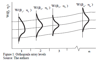
 ,
,  ,
,  and
and  (the ALTA Pro software was used). In addition, observe that although in Table 1 there are three level combinations among the variables, which as a consequence lead to three Weibull families in this DOE, regardless of this, in the standard approach [eq. (3)], only one shape parameter
  was estimated.
  , estimated by ML, and their associated reliability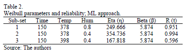
 in
in  (e.g. in Arrhenius
  ) and the corresponding logarithm of the scale parameter
 .
.  .
.  from the logarithm of
  for the operational (or desired) level (see next section). Finally, form the Weibull family of the operational (or desired) level W(
 ) with the shape parameters estimated in step1 and the scale parameter estimated in this step. And with these Weibull parameters, determine the desired reliability indexes.
 , thus the primitive (integral)
  of
of  , is given by
  . Since
 and
and  are the parameters to be estimated, and T is the absolute temperature (Kelvin). The linear form of (15a) is given by

 are given in Table 5b.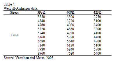
 and
and  with
with  . Finally, by using these parameters, the Weibull family mentioned in step 4, for a level of 323K is
  .
.
 , with primitive
  , thus
  . This formulation with
  is used in the Eyring model when the temperature is used. The Eyring model is given by:
 and
and  are parameters to be estimated and T is the absolute temperature. The linear relationship of (17) is


 and
and  with
with  . By using these parameters the Weibull family mentioned in step 4, for a level of 323K is
  .
.
 . This could be performed by ML, but MLR is recommended. (ML is a biased estimator and n is small).
 and the corresponding logarithm of the scale parameter
  .
.  by reordering (7a) as
 . In (20),
  is as in (7b), and
  and
and  are the shape parameter and the logarithm of the lifetime data of the i-th Weibull families of step 1.
  where
where  is the sample variance of the lifetime data, form the logarithm vector
 where
where  is the variance of the i-th level defined in (9c) and n is the number of replicates of the i-th level of step1.
 and
and  as the response variable and perform a regression between
  of the operational level, and by applying (14), with
  of step 1 and a desired
  value.
  are the parameters of the Weibull family of the desired stress level and they could be used to determine any desired reliability index. Observe that the estimation of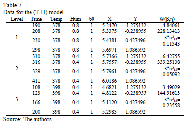
 and
and  ,
,  , and
, and  with
with  . The parameters of the regression between
  are
are  ,
,  and
and  with
with  . To show the method, suppose that the operational level is
  with
with  , then, by using the above parameters as in step 4,
  , and by taking
  ,
,  and
and  ,
,  . Thus, the operational Weibull family is
  .
. 
 ,
,  ,
,  with
with  and
and  . With operational Weibull Family given by
  . A comparison of the Weibull parameters and reliability index of the ML and the proposed Method is given in
 , thus the proposed method could easily be generalized to the right censured case by reflecting the censured data on
  for
for  in (9b) where