<?xml version="1.0" encoding="ISO-8859-1"?><article xmlns:mml="http://www.w3.org/1998/Math/MathML" xmlns:xlink="http://www.w3.org/1999/xlink" xmlns:xsi="http://www.w3.org/2001/XMLSchema-instance">
<front>
<journal-meta>
<journal-id>0012-7353</journal-id>
<journal-title><![CDATA[DYNA]]></journal-title>
<abbrev-journal-title><![CDATA[Dyna rev.fac.nac.minas]]></abbrev-journal-title>
<issn>0012-7353</issn>
<publisher>
<publisher-name><![CDATA[Universidad Nacional de Colombia]]></publisher-name>
</publisher>
</journal-meta>
<article-meta>
<article-id>S0012-73532016000400029</article-id>
<article-id pub-id-type="doi">10.15446/dyna.v83n198.51310</article-id>
<title-group>
<article-title xml:lang="en"><![CDATA[Multi-product inventory modeling with demand forecasting and Bayesian optimization]]></article-title>
<article-title xml:lang="es"><![CDATA[Modelo de inventario multi-producto, con pronósticos de demanda y optimización Bayesiana]]></article-title>
</title-group>
<contrib-group>
<contrib contrib-type="author">
<name>
<surname><![CDATA[Valencia-Cárdenas]]></surname>
<given-names><![CDATA[Marisol]]></given-names>
</name>
<xref ref-type="aff" rid="A01"/>
</contrib>
<contrib contrib-type="author">
<name>
<surname><![CDATA[Díaz-Serna]]></surname>
<given-names><![CDATA[Francisco Javier]]></given-names>
</name>
<xref ref-type="aff" rid="A02"/>
</contrib>
<contrib contrib-type="author">
<name>
<surname><![CDATA[Correa-Morales]]></surname>
<given-names><![CDATA[Juan Carlos]]></given-names>
</name>
<xref ref-type="aff" rid="A03"/>
</contrib>
</contrib-group>
<aff id="A01">
<institution><![CDATA[,Institución Universitaria Tecnológico de Antioquia  ]]></institution>
<addr-line><![CDATA[Medellín ]]></addr-line>
<country>Colombia</country>
</aff>
<aff id="A02">
<institution><![CDATA[,Universidad Nacional de Colombia Facultad de Minas ]]></institution>
<addr-line><![CDATA[Medellín ]]></addr-line>
<country>Colombia</country>
</aff>
<aff id="A03">
<institution><![CDATA[,Universidad Nacional de Colombia Facultad de Ciencias ]]></institution>
<addr-line><![CDATA[Medellín ]]></addr-line>
<country>Colombia</country>
</aff>
<pub-date pub-type="pub">
<day>00</day>
<month>09</month>
<year>2016</year>
</pub-date>
<pub-date pub-type="epub">
<day>00</day>
<month>09</month>
<year>2016</year>
</pub-date>
<volume>83</volume>
<numero>198</numero>
<fpage>235</fpage>
<lpage>243</lpage>
<copyright-statement/>
<copyright-year/>
<self-uri xlink:href="http://www.scielo.org.co/scielo.php?script=sci_arttext&amp;pid=S0012-73532016000400029&amp;lng=en&amp;nrm=iso"></self-uri><self-uri xlink:href="http://www.scielo.org.co/scielo.php?script=sci_abstract&amp;pid=S0012-73532016000400029&amp;lng=en&amp;nrm=iso"></self-uri><self-uri xlink:href="http://www.scielo.org.co/scielo.php?script=sci_pdf&amp;pid=S0012-73532016000400029&amp;lng=en&amp;nrm=iso"></self-uri><abstract abstract-type="short" xml:lang="en"><p><![CDATA[The complexity of supply chains requires advanced methods to schedule companies' inventories. This paper presents a comparison of model forecasts of demand for multiple products, choosing the best among the following: autoregressive integrated moving average (ARIMA), exponential smoothing (ES), a Bayesian regression model (BRM), and a Bayesian dynamic linear model (BDLM). To this end, cases in which the time series is normally distributed are first simulated. Second, sales predictions for three products of a gas service station are estimated using the four models, revealing the BRM to be the best model. Subsequently, the multi-product inventory model is optimized. To define the policies for ordering, inventory, costs, and profits, a Bayesian search integrating elements of a Tabu search is used to improve the solution. This inventory model optimization process is then applied to the case of a gas service station in Colombia.]]></p></abstract>
<abstract abstract-type="short" xml:lang="es"><p><![CDATA[La complejidad de las cadenas de suministro exige mejores métodos para programar los inventarios de una empresa. En este trabajo se presenta una comparación entre modelos de pronósticos de demanda de múltiples productos, eligiendo el mejor entre: ARIMA, Suavización exponencial, Regresión Lineal Bayesiana y un Modelo Lineal Dinámico Bayesiano. Para ello, primero se realiza una simulación de casos donde no hay una Distribución Normal en las series de tiempo, segundo, se estiman las predicciones de ventas de tres productos de una estación de servicios de gasolina con los cuatro modelos, encontrando los mejores resultados para la Regresión Lineal Bayesiana. Seguido a esto, se presenta la optimización de un Modelo de Inventarios Multi-Producto. Para definir la política de pedidos, inventarios, costos y ganancias, se utiliza una búsqueda bayesiana, que integra elementos de búsqueda Tabú para mejorar la solución. Dicha Optimización del Modelo de Inventarios se aplica a un caso de una estación de combustibles en Colombia.]]></p></abstract>
<kwd-group>
<kwd lng="en"><![CDATA[Dynamic Linear Models]]></kwd>
<kwd lng="en"><![CDATA[Inventory Models]]></kwd>
<kwd lng="en"><![CDATA[Forecasts]]></kwd>
<kwd lng="en"><![CDATA[Bayesian Statistics]]></kwd>
<kwd lng="es"><![CDATA[Modelos Dinámicos Lineales]]></kwd>
<kwd lng="es"><![CDATA[Modelos de Inventarios]]></kwd>
<kwd lng="es"><![CDATA[Pronósticos]]></kwd>
<kwd lng="es"><![CDATA[Estadística Bayesiana]]></kwd>
</kwd-group>
</article-meta>
</front><body><![CDATA[ <p><font size="1" face="Verdana, Arial, Helvetica, sans-serif"><b>DOI:</b> <a href="http://dx.doi.org/10.15446/dyna.v83n198.51310" target="_blank">http://dx.doi.org/10.15446/dyna.v83n198.51310</a></font></p>     <p align="center"><font size="4" face="Verdana, Arial, Helvetica, sans-serif"><b>Multi-product   inventory modeling with demand forecasting and Bayesian optimization</b></font></p>     <p align="center"><b><font size="3" face="Verdana, Arial, Helvetica, sans-serif"><i>Modelo   de inventario multi-producto, con pron&oacute;sticos de demanda y optimizaci&oacute;n   Bayesiana</i></font></b></p>     <p align="center">&nbsp;</p>     <p align="center"><b><font size="2" face="Verdana, Arial, Helvetica, sans-serif">Marisol Valencia-C&aacute;rdenas <i><sup>a</sup></i>,   Francisco Javier D&iacute;az-Serna <i><sup>b</sup></i> &amp; Juan Carlos Correa-Morales <i><sup>c</sup></i></font></b></p>     <p align="center">&nbsp;</p>     <p align="center"><font size="2" face="Verdana, Arial, Helvetica, sans-serif"><sup><i>a</i></sup><i> Instituci&oacute;n Universitaria Tecnol&oacute;gico de Antioquia, Medell&iacute;n, Colombia. <a href="mailto:mvalencia@unal.edu.co">mvalencia@unal.edu.co</a>    <br>   <sup>b </sup>Facultad de Minas, Universidad Nacional de Colombia, Medell&iacute;n, Colombia. <a href="mailto:javidiaz@unal.edu.co">javidiaz@unal.edu.co</a>    <br>   <sup>c </sup>Facultad de Ciencias, Universidad Nacional de Colombia, Medell&iacute;n,   Colombia. <a href="mailto:jccorrea@unal.edu.co">jccorrea@unal.edu.co</a></i><a href="mailto:jccorrea@unal.edu.co"></a></font></p>     <p align="center">&nbsp;</p>     ]]></body>
<body><![CDATA[<p align="center"><font size="2" face="Verdana, Arial, Helvetica, sans-serif"><b>Received: June 16<sup>th</sup>, 2015.   Received in revised form: November 1<sup>st</sup>, 2015. Accepted: July 25<sup>th</sup>,   2016.</b></font></p>     <p align="center">&nbsp;</p>     <p align="center"><font size="1" face="Verdana, Arial, Helvetica, sans-seriff"><b>This work is licensed under a</b> <a rel="license" href="http://creativecommons.org/licenses/by-nc-nd/4.0/">Creative Commons Attribution-NonCommercial-NoDerivatives 4.0 International License</a>.</font><br />   <a rel="license" href="http://creativecommons.org/licenses/by-nc-nd/4.0/"><img style="border-width:0" src="https://i.creativecommons.org/l/by-nc-nd/4.0/88x31.png" /></a></p> <hr>     <p><font size="2" face="Verdana, Arial, Helvetica, sans-serif"><b>Abstract    <br>   </b></font><font size="2" face="Verdana, Arial, Helvetica, sans-serif">The   complexity of supply chains requires advanced methods to schedule companies'   inventories. This paper presents a comparison of model forecasts of demand for   multiple products, choosing the best among the following: autoregressive   integrated moving average (ARIMA), exponential smoothing (ES), a Bayesian   regression model (BRM), and a Bayesian dynamic linear model (BDLM). To this   end, cases in which the time series is normally distributed are first   simulated. Second, sales predictions for three products of a gas service   station are estimated using the four models, revealing the BRM to be the best   model. Subsequently, the multi-product inventory model is optimized. To define   the policies for ordering, inventory, costs, and profits, a Bayesian search   integrating elements of a Tabu search is used to improve the solution. This   inventory model optimization process is then applied to the case of a gas   service station in Colombia.</font></p>     <p><font size="2" face="Verdana, Arial, Helvetica, sans-serif"><i>Keywords</i>: Dynamic Linear   Models, Inventory Models, Forecasts, Bayesian Statistics.</font></p>     <p><font size="2" face="Verdana, Arial, Helvetica, sans-serif"><b>Resumen    <br>   </b></font><font size="2" face="Verdana, Arial, Helvetica, sans-serif">La complejidad de las cadenas de suministro exige mejores m&eacute;todos para   programar los inventarios de una empresa. En este trabajo se presenta una   comparaci&oacute;n entre modelos de pron&oacute;sticos de demanda de m&uacute;ltiples productos,   eligiendo el mejor entre: ARIMA, Suavizaci&oacute;n exponencial, Regresi&oacute;n Lineal   Bayesiana y un Modelo Lineal Din&aacute;mico Bayesiano. Para ello, primero se realiza   una simulaci&oacute;n de casos donde no hay una Distribuci&oacute;n Normal en las series de   tiempo, segundo, se estiman las predicciones de ventas de tres productos de una   estaci&oacute;n de servicios de gasolina con los cuatro modelos, encontrando los   mejores resultados para la Regresi&oacute;n Lineal Bayesiana. Seguido a esto, se   presenta la optimizaci&oacute;n de un Modelo de Inventarios Multi-Producto. Para   definir la pol&iacute;tica de pedidos, inventarios, costos y ganancias, se utiliza una   b&uacute;squeda bayesiana, que integra elementos de b&uacute;squeda Tab&uacute; para mejorar la   soluci&oacute;n. Dicha Optimizaci&oacute;n del Modelo de Inventarios se aplica a un caso de   una estaci&oacute;n de combustibles en Colombia.</font></p>     <p><font size="2" face="Verdana, Arial, Helvetica, sans-serif"><i>Palabras clave</i>: Modelos Din&aacute;micos Lineales, Modelos de Inventarios,   Pron&oacute;sticos, Estad&iacute;stica Bayesiana.</font></p> <hr>     <p>&nbsp;</p>     ]]></body>
<body><![CDATA[<p><font size="3" face="Verdana, Arial, Helvetica, sans-serif"><b>1. Introduction</b></font></p>     <p><font size="2" face="Verdana, Arial, Helvetica, sans-serif">The increasing complexity of supply   chains resulting from the globalization of market economies, changes in   customer preferences, and increasing competition among companies is   intensifying the search for faster and better methods for decision-making and   obtaining optimal solutions for several types of inventory systems.</font></p>     <p><font size="2" face="Verdana, Arial, Helvetica, sans-serif">In   inventory models, as noted by Simchi-Levi &#91;1,2&#93;, demand represents a very important   variable that warrants substantial attention to determine adequate inventory   policies, and in some cases, the behavior of this variable is stochastic,   generating the need for accurate forecasting methods. However, problems can   arise because on occasion, the forecasting models are inappropriate or mistakes   are made, leading to error-laden inventory policies.</font></p>     <p><font size="2" face="Verdana, Arial, Helvetica, sans-serif">Other   problems associated with forecasting demand are related to changes in the   distribution function, which produce a lack of stability in the time series &#91;3&#93;; indeed, <i>&quot;… a time series is unstable if there are frequent and significant   changes in the distribution&quot; </i>&#91;3&#93;. This phenomenon has been cited by   different authors &#91;4-6&#93;. Other disadvantages are that,   sometimes, the models of interest cannot satisfy some theoretical assumptions,   such as normality in residuals or constant variance. Alternatively, the   researcher may not have sufficient required data for model estimation.</font></p>     <p><font size="2" face="Verdana, Arial, Helvetica, sans-serif">In this   sense, Bayesian statistics can be very good alternative for making inferences   using different types of models &#91;7-9&#93;, as shown for Bayesian forecasting   with the Holt winters model &#91;10&#93;, the dynamic models proposed in &#91;8,11&#93;, and especially, the situation   described in &#91;12&#93;, in which the authors describe   making forecasts in R using a package they developed. Other works report using   a combination of Bayesian techniques for forecasting &#91;13-15&#93;, and &#91;14&#93; reveals that using such combinations   results in increased accuracy and reliability. Bayesian forecasting has many   practical applications &#91;8,10,11,16-31&#93;. These methods constitute   alternatives to forecast and can be compared with classical methods to identify   ways to further increase the accuracy of the required predictions. </font></p>     <p><font size="2" face="Verdana, Arial, Helvetica, sans-serif">In addition   to the analytical techniques that can be used to solve inventory models, a   practical problem-solving approach exists that is known as heuristics.   Heuristics can be programmed according to some rules, but obtaining the optimal   solution for a model is not always guaranteed.</font></p>     <p><font size="2" face="Verdana, Arial, Helvetica, sans-serif">Some works   relating to inventory models have applied heuristic optimization. The Tabu   Search algorithm can be used to search for solutions to inventory problems; for   example, according to &#91;32&#93;, this algorithm was used to minimize   the inventory costs of an organization's final products and gave a better   result than the company policy. Indeed, when it was applied to a real situation   involving the same products with the same time horizon, it reduced inventory   costs by 20% while achieving a 100% service level. In &#91;33&#93;, the Tabu Search algorithm is   applied to determine the optimum level of orders. Genetic algorithms can be   used for efficient supply chain management &#91;34&#93; in multi-product scenarios, but such   scenarios are infrequently analyzed using inventory models. A recent work in   Colombia &#91;35&#93; proposed a model of multi-product   inventory between companies to minimize logistics costs in an urban   distribution operational context. In all of these cases, demand was predicted.   The measure symmetric mean absolute percentage error   (SMAPE), as described in &#91;36&#93;, is useful when the response takes values close to zero because   using it does not cause the error percentage to increase more when a response   is very small.</font></p>     <p><font size="2" face="Verdana, Arial, Helvetica, sans-serif">In their book <i>Dynamic </i>Linear<i> Models with R</i>, Petris et al. &#91;12&#93; demonstrate many applications and the use of the package dlm,   which they developed. They also list the error indicators used to compare   models: mean absolute percentage error (MAPE), mean absolute deviation (MAD)   and mean squared error (MSE) or root-mean-square error (RMSE).</font></p>     <p><font size="2" face="Verdana, Arial, Helvetica, sans-serif">In this paper, first, we report a   simulation study allowing the recreation and analysis of the behavior of a   demand time series with dynamic variation after finding an adequate model to   forecast these types of data. The compared models are as follows:   autoregressive integrated moving average (ARIMA); exponential smoothing (ES), a   novel model developed in a doctoral thesis &#91;37&#93;; a Bayesian regression model (BRM); and a modified Bayesian   dynamic linear model (BDLM) presented in that thesis in which a MAPE indicator   is used for the comparisons. In this paper, the estimated models are compared   using the SMAPE for forecasts once the data have been partitioned. Then, after   applying the best model to a real case of combustible demand for a Colombian   gas service station, the prediction is saved to do an optimization process. </font></p>     <p><font size="2" face="Verdana, Arial, Helvetica, sans-serif">Finally, we propose a multi-product   inventory model that provides not only orders, inventory values, costs, and   profits but also transportation durations and costs. The solutions obtained by   this optimization process are based on a search that utilizes a Bayesian form   to predict orders based on the previous forecasted demands. However, unlike   that described in the aforementioned thesis, here, no missing values are considered,   and the result for 15 days of planning is shown.</font></p>     ]]></body>
<body><![CDATA[<p>&nbsp;</p>     <p><font size="3" face="Verdana, Arial, Helvetica, sans-serif"><b>2. Demand forecasting </b></font></p>     <p><font size="2" face="Verdana, Arial, Helvetica, sans-serif">We consider   four models for making predictions: ARIMA, ES, BRM, and BDLM. For this purpose,   we program an algorithm using R software to choose the best possible forecast.</font></p>     <p><font size="2" face="Verdana, Arial, Helvetica, sans-serif">The   ARIMA(p,d,q) model, which was developed in 1970, by George Box and Gwilym   Jenkins &#91;38,39&#93; has been widely studied &#91;40-44&#93;. This model incorporates the   characteristics of the same time series according to the autocorrelation results   and makes predictions based on historical data.</font></p>     <p><font size="2" face="Verdana, Arial, Helvetica, sans-serif">ES is   another oft-used technique &#91;10,45,46&#93; that employs exponential weights of   past periods' values in the same series. This model can incorporate the level   of the time series, trend and seasonality and it is expressed as follows: <img src="/img/revistas/dyna/v83n198/v83n198a29eq002.gif">, where <img src="/img/revistas/dyna/v83n198/v83n198a29eq004.gif"> is the forecast for the next period, <font face="Symbol">a</font> is the smoothing constant, <img src="/img/revistas/dyna/v83n198/v83n198a29eq006.gif"> is the real value of the series in period t, and <img src="/img/revistas/dyna/v83n198/v83n198a29eq008.gif">is the predicted value for the period   t-1. The response variable <img src="/img/revistas/dyna/v83n198/v83n198a29eq006.gif"> is adjusted according to a time horizon, and   the sum of squared errors of prediction (SSE) value is optimized by searching   for the value of <font face="Symbol">a</font> that minimizes it. </font></p>     <p><font size="2" face="Verdana, Arial, Helvetica, sans-serif">Bayesian   statistics relies on different assumptions than classical models. For example,   the parameters of a probability distribution are random variables, q, and prior quantitative information is included   in a probability distribution &#91;47,48&#93; known as <img src="/img/revistas/dyna/v83n198/v83n198a29eq010.gif">, with simple information (y<sub>1</sub>,   y<sub>2</sub>, …, y<sub>n</sub>) summarized by the likelihood function L(y<sub>1</sub>,   y<sub>2</sub>, …, y<sub>n</sub> | q). Using the Bayes theorem-the a prior   distribution <img src="/img/revistas/dyna/v83n198/v83n198a29eq010.gif"> multiplied by the likelihood-gives the   posterior distribution <img src="/img/revistas/dyna/v83n198/v83n198a29eq012.gif">. The predictive distribution is the   integral of the distribution of the variable to be forecasted and the posterior   distribution &#91;49,50&#93;. </font></p>     <p><font size="2" face="Verdana, Arial, Helvetica, sans-serif"><b><i>2.1. Bayesian regression model (BRM)</i></b></font></p>     <p><font size="2" face="Verdana, Arial, Helvetica, sans-serif">In &#91;51&#93;, Zellner presents a BRM based on a   diffuse prior distribution of b parameters. In this work, a different   model will be presented: the novel BRM described in thesis above &#91;37&#93;. The model presented there assumes a   Normal prior distribution for the vector parameter b and applies an iterative process to   the initial vector b<sub>0</sub> for every time t; however, its accuracy   parameter is fixed: t<sub>0 </sub>= 1/<font face="Symbol">s</font>.<sub>, </sub>The predictive   distribution used for forecasting is derived in the thesis and is a Student's   t-distribution; this derivation is also presented in the appendix of this   paper.</font></p>     <p><font size="2" face="Verdana, Arial, Helvetica, sans-serif">The   general equation of a linear model is the same in a Bayesian regression, but   the estimation process is different. We describe this process here based on the   general equation given by eq. (1), where y<sub>t </sub>is the demand vector,   and <i>x<sub>1</sub>, …, x<sub>k</sub></i> are the explanatory variables. </font></p>     <p><img src="/img/revistas/dyna/v83n198/v83n198a29eq01.gif"></p>     ]]></body>

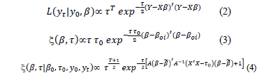
<body><![CDATA[<p><font size="2" face="Verdana, Arial, Helvetica, sans-serif">The likelihood function of   the data, based in the Normal distribution, is shown in eq. (2), a prior Normal   distribution for the b parameter vector, in eq. (3) and the posterior distribution is (4),   obtained after the product of the prior times the likelihood, and the algebraic   process. Here, <img src="/img/revistas/dyna/v83n198/v83n198a29eq016.gif">, and <img src="/img/revistas/dyna/v83n198/v83n198a29eq018.gif"></font></p>     <p><img src="/img/revistas/dyna/v83n198/v83n198a29eq0204.gif"></p>     <p><font size="2" face="Verdana, Arial, Helvetica, sans-serif">After taking the integral   of the product of the posterior and future data distributions, the resulting   predictive distribution is described by eq.   (5), which is a Student's t-distribution, with mean <img src="/img/revistas/dyna/v83n198/v83n198a29eq026.gif">, n degrees of freedom, and variance according to   eq. (6). The forecasting process uses the eq. (5), and its mean considers the   designed matrix <i>X</i> based on the   adjustment of the regression eq. (1). The analytical formulation of this   predictive distribution is also explained in the appendix.</font></p>     <p><img src="/img/revistas/dyna/v83n198/v83n198a29eq0506.gif"></p>     <p><font size="2" face="Verdana, Arial, Helvetica, sans-serif"><b><i>2.2. Bayesian dynamic linear model (BDLM) </i></b></font></p>     <p><font size="2" face="Verdana, Arial, Helvetica, sans-serif">In &#91;21&#93;, Meinhold and   Singpurwalla explain the process used to update <img src="/img/revistas/dyna/v83n198/v83n198a29eq032.gif"> in a recursive form using the posterior Normal   distribution to update the observed equation. The model proposed in this work   is based on the procedure described in the aforementioned thesis &#91;37&#93;, except that the mean value of the posterior   Normal distribution are modified based on an average of past values before   estimating the observation equation and without the M model used by Meinhold and Singpurwalla. The process is   included in the algorithm designed in the R program.</font></p>     <p><font size="2" face="Verdana, Arial, Helvetica, sans-serif"><b><i>2.3. Simulation of the forecasting process</i></b></font></p>     <p><font size="2" face="Verdana, Arial, Helvetica, sans-serif">We simulate different time   series under control conditions. For the simulated series, an estimation   process is executed using classical and Bayesian techniques. Subsequently, a   comparison is conducted using the SMAPE indicator. The objective is to   determine the best forecasting model to use if the time series exhibits high   variability and apply it to a real case to obtain predicted values useful for   developing and proposing an inventory policy.</font></p>     <p><font size="2" face="Verdana, Arial, Helvetica, sans-serif">The demands analyzed are   mainly of a continuous nature, but they do not always follow a Normal   distribution. The following cases are used to create the simulated time series:</font></p>     <blockquote>       ]]></body>
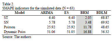
<body><![CDATA[<p align="left"><font size="2" face="Verdana, Arial, Helvetica, sans-serif">S1. Regression     model with skew Normal distribution for errors, with seasonal and dynamic     variation.    <br>     </font><font size="2" face="Verdana, Arial, Helvetica, sans-serif">S2. Regression     model with skew T-distribution for errors, with seasonal and dynamic variation.    <br>     </font><font size="2" face="Verdana, Arial, Helvetica, sans-serif">S3. Random     variable with Poisson distribution.    <br>     </font><font size="2" face="Verdana, Arial, Helvetica, sans-serif">S4. Random     variable with Poisson distribution and seasonal and dynamic variation.</font></p> </blockquote>     <p><font size="2" face="Verdana, Arial, Helvetica, sans-serif">The   size of each time series is N = 63 data points and a seasonal variation of   seven periods. Each time series consists of 49 data points for the adjustment   and 14 data points for forecasting. </font></p>     <p><font size="2" face="Verdana, Arial, Helvetica, sans-serif">The   SMAPE of the forecasted values is used as the criterion for identifying the   best model, and it is calculated with eq. (7) according to &#91;36&#93;, after estimating each of the four models being      compared: ARIMA, ES, BRM, and BDLM. </font></p>     <p><img src="/img/revistas/dyna/v83n198/v83n198a29eq07.gif"></p>     <p><font size="2" face="Verdana, Arial, Helvetica, sans-serif">where:</font></p>     <p><font size="2" face="Verdana, Arial, Helvetica, sans-serif"><img src="/img/revistas/dyna/v83n198/v83n198a29eq036.gif">: Forecasted value of the demand at   period t+1.</font></p>     <p><font size="2" face="Verdana, Arial, Helvetica, sans-serif"><img src="/img/revistas/dyna/v83n198/v83n198a29eq038.gif">: Real value of the demand at period   t+1.</font></p>     ]]></body>

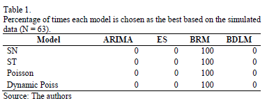
<body><![CDATA[<p><font size="2" face="Verdana, Arial, Helvetica, sans-serif">N : Total number of data points.</font></p>     <p><font size="2" face="Verdana, Arial, Helvetica, sans-serif">k : Total number of forecasted data points.</font></p>     <p><font size="2" face="Verdana, Arial, Helvetica, sans-serif">N-k : Total number of data points   used to adjust the model. </font></p>     <p><font size="2" face="Verdana, Arial, Helvetica, sans-serif">The   algorithms for the simulation were developed using the R program &#91;52&#93;. For the BRM, a vector of 200 percentile values   is calculated, and then, a prediction is made using the Student-t predictive   distribution. The error indicator SMAPE is calculated for the adjusted and   forecasted data for all models to facilitate finding the minimum SMAPE value. </font></p>     <p><font size="2" face="Verdana, Arial, Helvetica, sans-serif">This   process is repeated a thousand times, and the program calculates the percentage   of selection for every model and simulated case. The results of the frequency   with which each tested model is chosen as the best model are shown in <a href="#tab01">Table 1</a>. For   all simulated time series, the BRM is identified as the best model.</font></p>     <p align="center"><font size="2" face="Verdana, Arial, Helvetica, sans-serif"><a name="tab01"></a></font><img src="/img/revistas/dyna/v83n198/v83n198a29tab01.gif"></p>     <p><font size="2" face="Verdana, Arial, Helvetica, sans-serif"><a href="#tab02">Table   2</a> shows that, for one simulated case, as indicated by the grey color, lower   SMAPE values are found for the BRM in all analyzed cases. The results of the   two tables are consistent for all scenarios, confirming the reliability of the   results.</font></p>     <p align="center"><font size="2" face="Verdana, Arial, Helvetica, sans-serif"><a name="tab02"></a></font><img src="/img/revistas/dyna/v83n198/v83n198a29tab02.gif"></p>     <p><font size="2" face="Verdana, Arial, Helvetica, sans-serif">These   results show that when few data points with high variance are used, the BRM   model produces the minimum SMAPE values for all simulated series.</font></p>     <p><font size="2" face="Verdana, Arial, Helvetica, sans-serif">Up to this point, we have   shown that in forecasting, when no Normal behavior exists, the BRM is a very   good alternative, to the two common used classical models and the new BDLM   model, which failed to provide good results in any case. </font></p>     ]]></body>
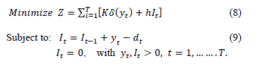
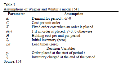
<body><![CDATA[<p>&nbsp;</p>     <p><font size="3" face="Verdana, Arial, Helvetica, sans-serif"><b>3. Multi-product inventory modeling</b></font></p>     <p><font size="2" face="Verdana, Arial, Helvetica, sans-serif"><b><i>3.1. Previous models </i></b></font></p>     <p><font size="2" face="Verdana, Arial, Helvetica, sans-serif">Some   classical inventory models were formulated based on Wagner and Whitin's proposed&#91;53&#93; cost minimization. These authors   specify that an order could be '0' or the sum of some demands, and they   formulated schemes for ordering (i.e., choosing between generating orders or   not) in every period t. </font></p>     <p><font size="2" face="Verdana, Arial, Helvetica, sans-serif">The model   formulated by Wagner   and Whitin, which is cited in &#91;54&#93;, assumes that a sequence of orders   over a planning horizon with a duration of T exists. The model assumptions are   shown in <a href="#tab03">Table 3</a>.</font></p>     <p><img src="/img/revistas/dyna/v83n198/v83n198a29eq0809.gif"></p>     <p><font size="2" face="Verdana, Arial, Helvetica, sans-serif">where the eq. (9) describes the   inventory-balance constraint for every period t.</font></p>     <p align="center"><font size="2" face="Verdana, Arial, Helvetica, sans-serif"><a name="tab03"></a></font><img src="/img/revistas/dyna/v83n198/v83n198a29tab03.gif"></p>     <p><font size="2" face="Verdana, Arial, Helvetica, sans-serif"><b><i>3.2. Proposed multi-product inventory model </i></b></font></p>     <p><font size="2" face="Verdana, Arial, Helvetica, sans-serif">A general   mathematical model of inventory management is formulated, and subsequently, an   optimization algorithm is developed.</font></p>     ]]></body>
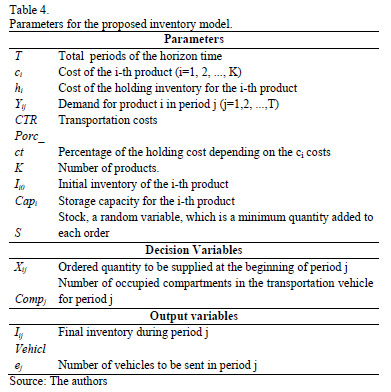
<body><![CDATA[<p><font size="2" face="Verdana, Arial, Helvetica, sans-serif">We propose   performing profit maximization using a formula similar to the Wagner-Within   model with the addition of transportation costs CTR<sub>t</sub>. Almost   equivalent results can be obtained by considering the problem as one of cost   minimization.</font></p>     <p align="center"><font size="2" face="Verdana, Arial, Helvetica, sans-serif"><a name="tab04"></a></font><img src="/img/revistas/dyna/v83n198/v83n198a29tab04.gif"></p>     <p><font size="2" face="Verdana, Arial, Helvetica, sans-serif">Objective function for the inventory   model.</font></p>     <p><img src="/img/revistas/dyna/v83n198/v83n198a29eq10.gif"></p>     <p><font size="2" face="Verdana, Arial, Helvetica, sans-serif">Subject to an inventory balance   constraint</font></p>     <p><img src="/img/revistas/dyna/v83n198/v83n198a29eq11.gif"></p>     <p><font size="2" face="Verdana, Arial, Helvetica, sans-serif">Capacity constrains for the orders</font></p>     <p><img src="/img/revistas/dyna/v83n198/v83n198a29eq12.gif"></p>     <p><font size="2" face="Verdana, Arial, Helvetica, sans-serif">The number of vehicles</font></p>     <p><img src="/img/revistas/dyna/v83n198/v83n198a29eq13.gif"></p>     ]]></body>
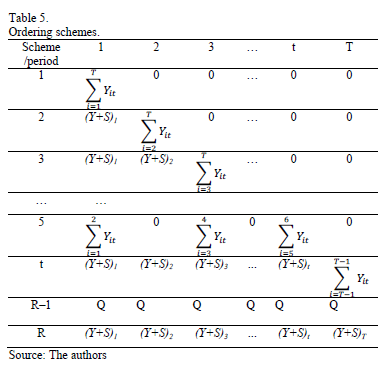
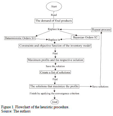
<body><![CDATA[<p><font size="2" face="Verdana, Arial, Helvetica, sans-serif">where <img src="/img/revistas/dyna/v83n198/v83n198a29eq056.gif"> represents the forecasted demand for product i   in period j. The transportation quantities and their respective costs will depend   on the number of vehicles to be used (<i>Vehicles<sub>t</sub></i>), which depend on the number of   compartments, <i>nc</i>, and these, depend   on those compartments' capacities, <i>Capc</i>,   assuming equal values. Dividing the quantity to order <i>x<sub>ij</sub></i> into <i>Capc,</i> generates a number of compartments, and the maximum integer value of this   number is divided into <i>nc</i>, producing   the total number of vehicles required, as represented by eq. (13), which can   then be substituted into the objective function shown in eq. (10).</font></p>     <p><font size="2" face="Verdana, Arial, Helvetica, sans-serif">The final inventory <img src="/img/revistas/dyna/v83n198/v83n198a29eq058.gif"> can be 0 or positive,   depending on the orders placed, as described in this work. The inventories are   limited by the storage capacity. Therefore, the orders cannot exceed that   capacity and can be equal to that maximum when there is zero inventory</font></p>     <p><font size="2" face="Verdana, Arial, Helvetica, sans-serif"><i>3.1.1. Algorithm</i></font></p>     <p><font size="2" face="Verdana, Arial, Helvetica, sans-serif">We describe the scenarios analyzed to   solve the proposed multi-product inventory model. The algorithm was programmed   in R software. </font></p>     <p><font size="2" face="Verdana, Arial, Helvetica, sans-serif">The schemes to order are of two kinds, S1   and S2, and the model was explained in the past section. These schemes are   replaced in the same model of the equations (10) to (13), and the best solution   is kept, in order to be compared and finding the maximum possible profits. The   process is repeated, and the random variable S, added to the orders (see <a href="#tab05">Table   5</a>), helps to find a best possible solution, after a period prepared to   simulate. </font></p>     <p align="center"><font size="2" face="Verdana, Arial, Helvetica, sans-serif"><a name="tab05"></a></font><img src="/img/revistas/dyna/v83n198/v83n198a29tab05.gif"></p>     <p><font size="2" face="Verdana, Arial, Helvetica, sans-serif">Two types of schemes are used for   ordering: S1 and S2; the model is described above. These schemes are   substituted into the model described by eqs. (10)-(13), and the best   solution is retained for posterior comparison and profit maximization with the   results obtained after the process repetition, by using the random variable S,   which is added to the orders (<a href="#tab05">Table 5</a>), and it facilitates finding the best   possible solution for the simulated period. </font></p>     <p><font size="2" face="Verdana, Arial, Helvetica, sans-serif">We calculate a maximum solution for each   S1-model and S2-model combination and save the best of them. After performing a   simulation of size &quot;<i>sim&quot;, </i>a list of   solutions is created, and   subsequently, the saved maximums are compared, the higher value is selected,   and the process is repeated until the best possible solution is obtained   according to the following convergence criterion: a difference of zero between <i>ten</i> consecutive values of <i>Z.</i></font></p>     <p><font size="2" face="Verdana, Arial, Helvetica, sans-serif">This process is presented in <a href="#fig01">Fig. 1</a>.</font></p>     <p align="center"><font size="2" face="Verdana, Arial, Helvetica, sans-serif"><a name="fig01"></a></font><img src="/img/revistas/dyna/v83n198/v83n198a29fig01.gif"></p>     ]]></body>
<body><![CDATA[<p><font size="2" face="Verdana, Arial, Helvetica, sans-serif">&bull; Ordering schemes </font></p>     <p><font size="2" face="Verdana, Arial, Helvetica, sans-serif">The first ordering   scheme, S1, is based on theorem 2 of &#91;53&#93;, which states that <i>&quot;there exists an optimal program such that   for all t&quot;:</i></font></p>     <p><img src="/img/revistas/dyna/v83n198/v83n198a29eq131.gif"></p>     <p><font size="2" face="Verdana, Arial, Helvetica, sans-serif">Thus, the formulation of S1 considers the   dynamics shown in <a href="#tab05">Table 5</a>. These R vectors of values are replaced in the model   described by eqs. (10)-(13), saving all of the equations and the   objective function, and finding the solution that maximizes the profits.</font></p>     <p><font size="2" face="Verdana, Arial, Helvetica, sans-serif">The second scheme, S2, generates orders   based on a predictive Bayesian distribution, as explained in section 3.2.2.   This allows a random variable based on the Bayesian process that depends on   previously forecasted demands to update the posterior distribution.   Subsequently, scheme S1 is used with random order values.</font></p>     <p><font size="2" face="Verdana, Arial, Helvetica, sans-serif">Ordering   schemes: Explanations corresponding   to <a href="#tab05">Table 5</a>:</font></p>     <blockquote>       <p><font size="2" face="Verdana, Arial, Helvetica, sans-serif">1. Ordering in the first period to     satisfy all the demands estimated for the planning horizon.    <br>     </font><font size="2" face="Verdana, Arial, Helvetica, sans-serif">2. Ordering in the first period to     satisfy only demand 1, and ordering in the second period to satisfy the sum of     the remaining demands.    <br>     </font><font size="2" face="Verdana, Arial, Helvetica, sans-serif">3. Ordering in the first two periods,     and ordering in the third period to satisfy the sum of the remaining demands.    ]]></body>
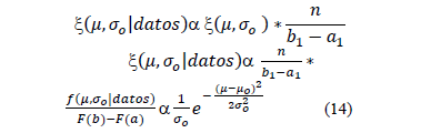
<body><![CDATA[<br>     </font><font size="2" face="Verdana, Arial, Helvetica, sans-serif">4. Same as 2 and 3 for resting periods,     until T-1; no ordering in the T-th period.    <br>     </font><font size="2" face="Verdana, Arial, Helvetica, sans-serif">5. Ordering every two periods.    <br>     </font><font size="2" face="Verdana, Arial, Helvetica, sans-serif">6. Ordering every three periods.    <br>     </font><font size="2" face="Verdana, Arial, Helvetica, sans-serif">7. Ordering every four periods and so     on.    <br>     </font><font size="2" face="Verdana, Arial, Helvetica, sans-serif">8. Ordering the economic order quantity     (EOQ).    <br>     </font><font size="2" face="Verdana, Arial, Helvetica, sans-serif">M. Ordering in all periods.</font></p> </blockquote>     <p><font size="2" face="Verdana, Arial, Helvetica, sans-serif"><i>3.1.2. Bayesian optimization</i></font></p>     <p><font size="2" face="Verdana, Arial, Helvetica, sans-serif">This is the procedure involving the   second scheme proposed (S2). The assumptions of this process are as follows: </font></p>     <p><font size="2" face="Verdana, Arial, Helvetica, sans-serif">The data distribution is uniform   (Data-unif(a1,b1)). Let '<font face="Symbol">m</font>' be the mean value of this distribution, with a   prior Normal truncated distribution with the following parameters: µo, mean; s<sub>o</sub>, standard deviation (assumed to be   constant); a, inferior limit; and b: superior limit (10).</font></p>     <p><img src="/img/revistas/dyna/v83n198/v83n198a29eq132.gif"></p>     ]]></body>
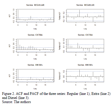
<body><![CDATA[<p><font size="2" face="Verdana, Arial, Helvetica, sans-serif">The product of the prior distribution and   the likelihood function is the Truncated Normal (TN), that is, the posterior   distribution (eq. (14)) of the mean parameters of the final predictive   distribution.</font></p>     <p><img src="/img/revistas/dyna/v83n198/v83n198a29eq14.gif"></p>     <p><font size="2" face="Verdana, Arial, Helvetica, sans-serif">The predictive distribution is the   integral of the Uniform distribution of the data and the posterior TN (14).   This distribution is uniform (15) and is used for forecasting, after updating   the means, with the posterior distribution for every time t.</font></p>     <p><img src="/img/revistas/dyna/v83n198/v83n198a29eq15.gif"></p>     <p>&nbsp;</p>     <p><font size="3" face="Verdana, Arial, Helvetica, sans-serif"><b>4. Results</b></font></p>     <p><font size="2" face="Verdana, Arial, Helvetica, sans-serif"><b><i>4.1. Comparison of the forecast results obtained using a real case</i></b></font></p>     <p><font size="2" face="Verdana, Arial, Helvetica, sans-serif">The dataset of the fuel sales includes 92   daily values for each product: Regular, Extra, and Diesel. In total, 77 data   points will be used to adjust the models, and 15 data points will be used for   forecasting. The last forecasted values will be used to optimize the models.   For the BRM, a vector of 200 percentiles was used to identify the best possible   position of the predictive Student T-distribution based on the minimum SMAPE   value of the 15 forecasts.</font></p>     <p><font size="2" face="Verdana, Arial, Helvetica, sans-serif">In the description of the Regular and   Diesel combustibles, the behavior seems to have a seasonal pattern with   seventh-order dependence, whereas for Extra, the behavior of the   autocorrelation shows a dependence of first order (<a href="#fig02">Fig. 2</a>), and it also shows seasonality   every 7 periods (days). These aspects are considered to estimate the models and   are used to define covariables to represent these behaviors.</font></p>     <p align="center"><font size="2" face="Verdana, Arial, Helvetica, sans-serif"><a name="fig02"></a></font><img src="/img/revistas/dyna/v83n198/v83n198a29fig02.gif"></p>     ]]></body>
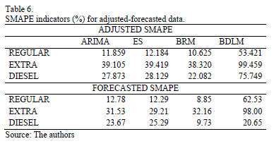
<body><![CDATA[<p><font size="2" face="Verdana, Arial, Helvetica, sans-serif">We also found that the residuals of the   ARIMA models estimated do not follow the normality assumption.</font></p>     <p><font size="2" face="Verdana, Arial, Helvetica, sans-serif">&bull; Description of the time series   analysis</font></p>     <p><font size="2" face="Verdana, Arial, Helvetica, sans-serif"><a href="#fig02">Fig. 2</a> presents the autocorrelation and   partial autocorrelation functions (ACF and PACF, respectively), they show that   the time series exhibits dependence of different orders (i.e., Regular, Extra   and Diesel fuels).</font></p>     <p><font size="2" face="Verdana, Arial, Helvetica, sans-serif"><a href="#tab06">Table 6</a> presents the adjusted and   forecasted SMAPE indicators (adjusted-forecasted), when the criterion used to   make a choice is based on one of these. Some advantages of the BRM models are   clearly evident.</font></p>     <p align="center"><font size="2" face="Verdana, Arial, Helvetica, sans-serif"><a name="tab06"></a></font><img src="/img/revistas/dyna/v83n198/v83n198a29tab06.gif"></p>     <p><font size="2" face="Verdana, Arial, Helvetica, sans-serif">According to the adjustment criteria, the   BRM is the best at forecasting the three products. Additionally, among the   forecasted values, the BRM produces the best results for Regular and Diesel   fuels, whereas for Extra, the ES is better, followed by ARIMA (it should be   noted that ARIMA's result is close to that of the BRM). The minimum adjustment   criterion is important because a researcher interested in forecasting would not   be able to choose the future data. Indeed, when the BRM is selected, the   probability of obtaining good performance is high. This approach leads us   choose the BRM as the model to forecast to these time series.</font></p>     <p><font size="2" face="Verdana, Arial, Helvetica, sans-serif">The results obtained by applying the   optimization process to a 15-day time horizon of fuel distribution and   inventory planning are presented below.</font></p>     <p><font size="2" face="Verdana, Arial, Helvetica, sans-serif"><b><i>4.2. Optimization of the application of the inventory model to a real case</i></b></font></p>     <p><font size="2" face="Verdana, Arial, Helvetica, sans-serif">If there were no holding costs and if the   inventory capacity were very high, the optimum strategy would be to send all   the demand for the T periods on the first day.</font></p>     <p><font size="2" face="Verdana, Arial, Helvetica, sans-serif">However, based on the real cost and   capacity data, the results obtained depend on the state of the initial   inventories. The designed algorithm compares the four combination models   proposed and requires no more than 1 minute to produce results when the initial   inventories exceed zero:</font></p> <ul>       ]]></body>
<body><![CDATA[<li><font size="2" face="Verdana, Arial, Helvetica, sans-serif">When the initial inventories     are set according to real data (4300, 1000, and 2150 gallons of Regular, Extra,     and Diesel, respectively), the maximum profit is $69,432.115, and the orders     are not sent every day. Instead, Regular fuel orders are sent on days 4, 7, 8,     10, 11 and 13, and Extra fuel orders are sent on days 7, 10 and 13. The model     did not indicate that sending diesel fuel was necessary because of the initial     inventory. </font></li>       <li><font size="2" face="Verdana, Arial, Helvetica, sans-serif">When the initial inventories     are all equal to zero, the optimal profit is $12,737.930. However, companies     typically prefer to have non-zero initial inventories.</font></li>     </ul>     <p><font size="2" face="Verdana, Arial, Helvetica, sans-serif"><b><i>4.3. Validation</i></b></font></p> <ul>       <li><font size="2" face="Verdana, Arial, Helvetica, sans-serif">Using real data, the profits     were $30,334.447 for a 15-day planning period.</font></li>       <li><font size="2" face="Verdana, Arial, Helvetica, sans-serif">Using the model proposed here,     with current initial inventories for each fuel (4300, 1000, and 2150 gallons of     Regular, Extra, and Diesel fuel, respectively) and by substituting the planned     orders for the real sales, the profits are $53,619.824, which is higher than     the original value. This difference represents a saving of 58.7% relative to     the current situation ($30,334.447).</font></li>     </ul>     <p><font size="2" face="Verdana, Arial, Helvetica, sans-serif">This result   shows that the model can provide a better solution for inventory management   than what was achieved in the real case.</font></p>     <p>&nbsp;</p>     <p><font size="3" face="Verdana, Arial, Helvetica, sans-serif"><b>5. Discussion</b></font></p>     ]]></body>
<body><![CDATA[<p><font size="2" face="Verdana, Arial, Helvetica, sans-serif">The proposed Bayesian forecasting methods   establish various accurate alternatives for making predictions compared to some   classical methods, such as ARIMA and ES. The modified version of the BRM   proposed in the aforementioned thesis &#91;37&#93; (in this case, the SMAPE indicator is used) was capable of   generating satisfactory results, as was also shown using MAPE in the thesis.</font></p>     <p><font size="2" face="Verdana, Arial, Helvetica, sans-serif">This alternative Bayesian method can be   improved by altering its parameters or probability distributions to obtain more   accurate values, which would result in a better optimization solution.   Additionally, different research lines could potentially benefit from this   optimization technique, which can also be applied to the Dynamic Linear Models   described by other authors, including Petris, Harrison and Stevens, and   Harrison and West &#91;8,9,11&#93;.</font></p>     <p>&nbsp;</p>     <p><font size="3" face="Verdana, Arial, Helvetica, sans-serif"><b>6. Conclusions</b></font></p>     <p><font size="2" face="Verdana, Arial, Helvetica, sans-serif">In addition   to maximizing its profits, the proposed inventory model could also consider the   fuel transportation costs incurred by the gas service station, and it functions   a very good planning tool, especially compared to other models, such as EOQ,   which was not found to be the best model in any case. Transportation costs   change in every period, and it is not necessary to send vehicles every day.   This model also revealed that sending all of the 15-day demands at the   beginning of each period was non-optimal, since these quantities involved could   exceed the available storage capacities. Furthermore, the model indicated that,   if the related costs were zero and the capacity were very high, satisfying all   the demands of the T periods during the first period would be optimal.</font></p>     <p>&nbsp;</p>     <p><font size="3" face="Verdana, Arial, Helvetica, sans-serif"><b>Appendix</b></font></p>     <p><font size="2" face="Verdana, Arial, Helvetica, sans-serif">Here, we show the transformation of the   exponent in eq. (4) to obtain the predictive Student T-distribution (5).</font></p>     <p><font size="2" face="Verdana, Arial, Helvetica, sans-serif"> <img src="/img/revistas/dyna/v83n198/v83n198a29eq090.gif"></font></p>     <p align=left><font size="2" face="Verdana, Arial, Helvetica, sans-serif"><i>Where </i><img src="/img/revistas/dyna/v83n198/v83n198a29eq092.gif"><i>, and </i><img src="/img/revistas/dyna/v83n198/v83n198a29eq094.gif"><i>. The exponent can also be expressed as:</i></font></p>     ]]></body>
<body><![CDATA[<p><font size="2" face="Verdana, Arial, Helvetica, sans-serif"><i>I = Y'<sub>+</sub>Y<sub>+</sub>-b'<sub>n</sub> M b<sub>n</sub> +Y'Y +b &quot;<sub>0</sub>t<sub>0</sub>b<sub>0</sub></i></font></p>     <p><font size="2" face="Verdana, Arial, Helvetica, sans-serif"><i>Where M<sup>-1</sup> = (X'<sub>+</sub>X<sub>+</sub> + X'X + t<sub>0</sub>)<sup>-1</sup>, and b<sub>n</sub> = M<sup>-1</sup>(X'Y + X'<sub>+</sub>Y + b<sub>0</sub>t<sub>0</sub>)</i></font></p>     <p><font size="2" face="Verdana, Arial, Helvetica, sans-serif"><i>I = Y'<sub>+</sub>Y<sub>+</sub>- M<sup>-1</sup>(X'Y + X'<sub>+</sub>Y<sub>+</sub> + b<sub>0</sub>t<sub>0</sub>)M M<sup>-1</sup>(X'Y   + X<sup>&quot;</sup><sub>+</sub>Y<sub>+ </sub>+ b<sub>0</sub>t<sub>0</sub>) + Y'Y + b'<sub>0</sub>t<sub>0</sub>b<sub>0 </sub></i> </font></p>     <p><font size="2" face="Verdana, Arial, Helvetica, sans-serif"><i>I = Y'<sub>+</sub>Y<sub>+ </sub>+ Y'Y + b<sup>'</sup><sub>0</sub>t<sub>0</sub>b<sub>0 </sub>- M<sup>-1</sup>&#91;(X<sup>&quot;</sup>Y)<sup>&quot;</sup>(X<sup>&quot;</sup>Y) </i></font></p>     <p><font size="2" face="Verdana, Arial, Helvetica, sans-serif"><i>+ (X<sup>&quot;</sup><sub>+</sub>Y<sub>+</sub>)<sup>&quot;</sup>(X<sup>&quot;</sup><sub>+</sub>Y<sub>+</sub>) + (b<sub>0</sub>t<sub>0</sub>)<sup>&quot;</sup>b<sub>0</sub>t<sub>0 </sub>+ 2(X'Y)'(X'<sub>+</sub>Y<sub>+</sub>) +</i></font></p>     <p><font size="2" face="Verdana, Arial, Helvetica, sans-serif"><i> 2(X<sup>&quot;</sup>Y)<sup>&quot;</sup>(b<sub>0</sub>t<sub>0</sub>) + 2(X'<sub>+</sub>Y<sub>+</sub>)<sup>&quot;</sup>(b<sub>0</sub>t<sub>0</sub>)&#93;</i></font></p>     <p><font size="2" face="Verdana, Arial, Helvetica, sans-serif"><i>I = Y<sub>+</sub>(I-X<sub>+</sub>M<sup>-1</sup>X<sub>+</sub>)Y<sub>+ </sub>-</i> <i>2Y<sub>+</sub>X<sub>+</sub>M<sup>-1</sup>(X<sup>&quot;</sup>Y + b<sub>0</sub>t<sub>0</sub>) + b<sup>&quot;</sup><sub>0</sub>t<sub>0</sub>b<sub>0 </sub>- M<sup>-1</sup>(Y X<sup>&quot;</sup>X<sup>&quot;</sup>Y + t<sub>0</sub>b'<sub>0</sub></i> <i>b<sub>0</sub>t<sub>0 </sub>+ 2X<sup>&quot;</sup>Y b<sub>0</sub>t<sub>0</sub>) + Y'Y</i></font></p>     <p><font size="2" face="Verdana, Arial, Helvetica, sans-serif"><i>I = &#91;Y<sub>+</sub>Y<sub>+</sub>- 2Y<sub>+</sub>X<sub>+</sub>(I - M<sup>-1</sup>X&quot;<sub>+</sub>X<sub>+</sub>)<sup>-1</sup>M<sup>-1</sup>(X&quot;Y   + b<sub>0</sub>t<sub>0</sub>)&#93;*</i></font></p>     <p><font size="2" face="Verdana, Arial, Helvetica, sans-serif"><i>(1 - M<sup>-1</sup>X&quot;<sub>+</sub>X&quot;<sub>+</sub>) + (b'<sub>0</sub>t<sub>0</sub>b<sub>0 </sub>- M<sup>-1</sup>t<sub>0</sub>b'<sub>0</sub></i> <i>b<sub>0</sub>t<sub>0</sub>) + (Y'(I - M<sup>-1</sup>X<sup>&quot;</sup>X)Y - 2M<sup>-1</sup>X<sup>&quot;</sup>Y b<sub>0</sub>t<sub>0</sub>)</i></font></p>     <p><font size="2" face="Verdana, Arial, Helvetica, sans-serif"><i>I = &#91;(Y<sub>+</sub>- Yn)&quot;(Y<sub>+</sub>- Y<sub>n</sub>) - Yn&quot;Yn&#93;(1 - M<sup>-1</sup>X&quot;<sub>+</sub>X&quot;<sub>+</sub>)   +</i></font></p>     ]]></body>
<body><![CDATA[<p><font size="2" face="Verdana, Arial, Helvetica, sans-serif"><i>(b'<sub>0</sub>t<sub>0</sub>b<sub>0 </sub>-</i> <i>M<sup>-1</sup>t<sub>0</sub>b'<sub>0</sub>b<sub>0</sub>t<sub>0</sub>) </i></font></p>     <p><font size="2" face="Verdana, Arial, Helvetica, sans-serif"><i>+ (Y&quot;Y - 2M<sup>-1</sup>(I - M<sup>-1</sup>X&quot;X)<sup>-1</sup>X&quot;Y b<sub>0</sub>t<sub>0</sub>)(I - M<sup>-1</sup>X&quot;X)</i></font></p>     <p><font size="2" face="Verdana, Arial, Helvetica, sans-serif"><i>I = &#91;(Y<sub>+</sub>- Y<sub>n</sub>)&quot;(Y<sub>+</sub>- Y<sub>n</sub>) - Y<sub>n</sub>&quot;Y<sub>n</sub>&#93;(1 - M<sup>-1</sup>X&quot;<sub>+</sub>X&quot;<sub>+</sub>)   +</i></font></p>     <p><font size="2" face="Verdana, Arial, Helvetica, sans-serif"><i>(b<sup>'</sup><sub>0</sub>t<sub>0</sub>b<sub>0 </sub>- M<sup>-1</sup>t<sub>0</sub>b'<sub>0</sub></i> <i>b<sub>0</sub>t<sub>0</sub>)</i></font></p>     <p><font size="2" face="Verdana, Arial, Helvetica, sans-serif"><i>+ &#91;(Y - Y<sub>m</sub>)&quot;(Y - Y<sub>m</sub>) - Y'<sub>m</sub>Y<sub>m</sub>&#93;   (I - M<sup>-1</sup>X&quot;X)</i></font></p>     <p><font size="2" face="Verdana, Arial, Helvetica, sans-serif"><i>Where Y<sub>n</sub> = (I - X<sub>+</sub>M<sup>-1</sup>X<sub>+</sub>)<sup>-1</sup>X<sub>+</sub>M<sup>-1</sup>(X<sup>&quot;</sup>Y + b<sub>0</sub>t<sub>0</sub>), according to a definition of inverted difference in matrices </i>&#91;51&#93;<i>.</i></font></p>     <p><font size="2" face="Verdana, Arial, Helvetica, sans-serif"><i>Y<sub>n</sub> = (I + X<sub>+</sub>(X<sup>&quot;</sup>X)<sup>-1</sup>X<sub>+</sub>)M<sup>-1</sup>X <sub>+ </sub>(X<sup>&quot;</sup>Y + b<sub>0</sub>t<sub>0</sub>)</i></font></p>     <p><font size="2" face="Verdana, Arial, Helvetica, sans-serif"><i>Therefore, Y<sub>n</sub> = (I + (X'X)<sup>-1</sup>X'<sub>+</sub>X<sub>+</sub>)(X<sup>&quot;</sup>X + t + X<sup>&quot;</sup><sub>+</sub>X<sub>+</sub>)<sup>-1</sup>X<sub>+</sub>(X<sup>&quot;</sup>Y + b<sub>0</sub>t<sub>0</sub>) </i></font></p>     <p><font size="2" face="Verdana, Arial, Helvetica, sans-serif"><i>=   (I + (X<sup>&quot;</sup>X)<sup>-1</sup>X<sup>'</sup><sub>+</sub>X<sub>+</sub>)(I + (X<sup>&quot;</sup>X+ t<sub>0</sub>)<sup>-1</sup>X'<sub>+</sub>X<sub>+</sub>)<sup>-1</sup>X<sub>+</sub> (X'X + t<sub>0</sub>)<sup>-1</sup>(X<sup>&quot;</sup>Y + b<sub>0</sub>t<sub>0</sub>)</i></font></p>     <p><font size="2" face="Verdana, Arial, Helvetica, sans-serif"><i>t<sub>0</sub> is a very small quantity. Thus, Y<sub>n</sub> = (X<sup>&quot;</sup>X + t<sub>0</sub>)<sup>-1</sup>X<sub>+</sub>(X<sup>&quot;</sup>Y + b<sub>0</sub>t<sub>0</sub>) = </i><img src="/img/revistas/dyna/v83n198/v83n198a29eq096.gif"> <i>, and</i></font></p>     ]]></body>
<body><![CDATA[<p><font size="2" face="Verdana, Arial, Helvetica, sans-serif"><img src="/img/revistas/dyna/v83n198/v83n198a29eq098.gif"><i>. Let Y<sub>m</sub> = M<sup>-1</sup>(I - M<sup>-1</sup>X'X )<sup> -1</sup>X'b<sub>0</sub>t<sub>0</sub></i></font></p>     <p><font size="2" face="Verdana, Arial, Helvetica, sans-serif">Some terms   disappear because of the proportionality:</font></p>     <p><font size="2" face="Verdana, Arial, Helvetica, sans-serif"><i>I = &#91;(Y<sub>+</sub>- Y<sub>n</sub>)'(Y<sub>+</sub>- Yn) - Yn'Yn&#93;(1 - M<sup>-1</sup>X'<sub>+</sub>X<sub>+</sub>)   + &#91;(Y - Ym)&quot;(Y - Ym) - YmYm&#93;(I - M<sup>-1</sup>X&quot;X) </i></font></p>     <p><font size="2" face="Verdana, Arial, Helvetica, sans-serif"><i>I = &#91;(Y<sub>+</sub>- Yn)'(Y<sub>+</sub>- Yn) + (Y - Ym)'(Y - Ym)</i></font></p>     <p><font size="2" face="Verdana, Arial, Helvetica, sans-serif"><img src="/img/revistas/dyna/v83n198/v83n198a29eq100.gif"> </font></p>     <p><font size="2" face="Verdana, Arial, Helvetica, sans-serif"><img src="/img/revistas/dyna/v83n198/v83n198a29eq102.gif"></font></p>     <p><font size="2" face="Verdana, Arial, Helvetica, sans-serif">which is the   Student t-distribution described by eq. (5).</font></p>     <p>&nbsp;</p>     <p><font size="3" face="Verdana, Arial, Helvetica, sans-serif"><b>Acknowledgments</b></font></p>     <p><font size="2" face="Verdana, Arial, Helvetica, sans-serif">Colciencias is acknowledged for providing   a scholarship (567) in support of obtaining a Doctorate in Engineering-Industry   and Organizations at Universidad Nacional de Colombia, Sede Medell&iacute;n.</font></p>     ]]></body>
<body><![CDATA[<p>&nbsp;</p>     <p><font size="3" face="Verdana, Arial, Helvetica, sans-serif"><b>References</b></font></p>     <!-- ref --><p><font size="2" face="Verdana, Arial, Helvetica, sans-serif"><b>&#91;1&#93;</b> Simchi-Levi,   D., Kaminski, P. and Simchi-Levi, E., Designing   and managing the supply chain. 3rd ed. New York: McGraw-Hill; 2008.    &nbsp;&nbsp;&nbsp;&nbsp;&nbsp;&nbsp;&nbsp;&nbsp;[&#160;<a href="javascript:void(0);" onclick="javascript: window.open('/scielo.php?script=sci_nlinks&ref=1151583&pid=S0012-7353201600040002900001&lng=','','width=640,height=500,resizable=yes,scrollbars=1,menubar=yes,');">Links</a>&#160;]<!-- end-ref --> </font></p>     <!-- ref --><p><font size="2" face="Verdana, Arial, Helvetica, sans-serif"><b>&#91;2&#93;</b> Chen, X. and Simchi-Levi, D., Coordinating inventory control   and pricing strategies with random demand and fixed ordering cost: The finite   horizon case. Operations Research, 2004, 52(6), pp. 887-896. DOI: 10.1287/opre.1040.0127</font>&nbsp;&nbsp;&nbsp;&nbsp;&nbsp;&nbsp;&nbsp;&nbsp;[&#160;<a href="javascript:void(0);" onclick="javascript: window.open('/scielo.php?script=sci_nlinks&ref=1151585&pid=S0012-7353201600040002900002&lng=','','width=640,height=500,resizable=yes,scrollbars=1,menubar=yes,');">Links</a>&#160;]<!-- end-ref --><!-- ref --><p><font size="2" face="Verdana, Arial, Helvetica, sans-serif"><b>&#91;3&#93;</b> Hillier, F. y Hillier, M., M&eacute;todos   cuantitativos para administraci&oacute;n. Third Ed. City: M&eacute;xico. McGraw-Hill; 2007.    &nbsp;&nbsp;&nbsp;&nbsp;&nbsp;&nbsp;&nbsp;&nbsp;[&#160;<a href="javascript:void(0);" onclick="javascript: window.open('/scielo.php?script=sci_nlinks&ref=1151586&pid=S0012-7353201600040002900003&lng=','','width=640,height=500,resizable=yes,scrollbars=1,menubar=yes,');">Links</a>&#160;]<!-- end-ref --> </font></p>     <!-- ref --><p><font size="2" face="Verdana, Arial, Helvetica, sans-serif"><b>&#91;4&#93;</b> Garcia,   C.A., Ibeas, A., Vilanova, R. and Herrera, J., Inventory control of supply   chains: Mitigating the bullwhip effect by centralized and decentralized   internal model control approaches. European   Journal of Operational Research, 224(2),   pp. 261-272, 2013. DOI: 10.1016/J.EJOR.2012.07.029</font>&nbsp;&nbsp;&nbsp;&nbsp;&nbsp;&nbsp;&nbsp;&nbsp;[&#160;<a href="javascript:void(0);" onclick="javascript: window.open('/scielo.php?script=sci_nlinks&ref=1151588&pid=S0012-7353201600040002900004&lng=','','width=640,height=500,resizable=yes,scrollbars=1,menubar=yes,');">Links</a>&#160;]<!-- end-ref --><!-- ref --><p><font size="2" face="Verdana, Arial, Helvetica, sans-serif"><b>&#91;5&#93;</b> Sarimveis,   H., Patrinos, P., Tarantilis, C.D. and Kiranoudis, C.T., Dynamic modeling and   control of supply chain systems: A review. Computers and Operations Research. 35(11), pp. 3530-3561, 2008. DOI: 10.1016/J.COR.2007.01.017</font>&nbsp;&nbsp;&nbsp;&nbsp;&nbsp;&nbsp;&nbsp;&nbsp;[&#160;<a href="javascript:void(0);" onclick="javascript: window.open('/scielo.php?script=sci_nlinks&ref=1151589&pid=S0012-7353201600040002900005&lng=','','width=640,height=500,resizable=yes,scrollbars=1,menubar=yes,');">Links</a>&#160;]<!-- end-ref --><!-- ref --><p><font size="2" face="Verdana, Arial, Helvetica, sans-serif"><b>&#91;6&#93;</b> Braun,   M.W., Rivera, D.E., Flores, M.E., Carlyle, W.M. and Kempf, K.G., A model   predictive control framework for robust management of multi-product,   multi-echelon demand networks. Annual   Reviews in Control, 27(2),   pp. 229-245, 2003. DOI:   10.1016/j.arcontrol.2003.09.006</font>&nbsp;&nbsp;&nbsp;&nbsp;&nbsp;&nbsp;&nbsp;&nbsp;[&#160;<a href="javascript:void(0);" onclick="javascript: window.open('/scielo.php?script=sci_nlinks&ref=1151590&pid=S0012-7353201600040002900006&lng=','','width=640,height=500,resizable=yes,scrollbars=1,menubar=yes,');">Links</a>&#160;]<!-- end-ref --><!-- ref --><p><font size="2" face="Verdana, Arial, Helvetica, sans-serif"><b>&#91;7&#93;</b> Pole,   A., West, M. and Harrison, J., Nonnormal and nonlinear dynamic Bayesian   modeling. In Bayesian analysis of time   series and dynamic linear models. New York: Marcel Dekker; 1988, pp.   167-198.    &nbsp;&nbsp;&nbsp;&nbsp;&nbsp;&nbsp;&nbsp;&nbsp;[&#160;<a href="javascript:void(0);" onclick="javascript: window.open('/scielo.php?script=sci_nlinks&ref=1151591&pid=S0012-7353201600040002900007&lng=','','width=640,height=500,resizable=yes,scrollbars=1,menubar=yes,');">Links</a>&#160;]<!-- end-ref --> </font></p>     <!-- ref --><p><font size="2" face="Verdana, Arial, Helvetica, sans-serif"><b>&#91;8&#93;</b> West,   M. and Harrison, J., Bayesian   forecasting and dynamic models. Second ed. New York: Springer Series in   Statistics; 1997.    &nbsp;&nbsp;&nbsp;&nbsp;&nbsp;&nbsp;&nbsp;&nbsp;[&#160;<a href="javascript:void(0);" onclick="javascript: window.open('/scielo.php?script=sci_nlinks&ref=1151593&pid=S0012-7353201600040002900008&lng=','','width=640,height=500,resizable=yes,scrollbars=1,menubar=yes,');">Links</a>&#160;]<!-- end-ref --> </font></p>     <!-- ref --><p><font size="2" face="Verdana, Arial, Helvetica, sans-serif"><b>&#91;9&#93;</b> Petris,   G., An R package for dynamic linear models. Journal of Statistical Software &#91;online&#93;, 36(12), pp. 1-16, 2010. Available at: <a href="http://www.jstatsoft.org/" target="_blank">http://www.jstatsoft.org/</a></font>&nbsp;&nbsp;&nbsp;&nbsp;&nbsp;&nbsp;&nbsp;&nbsp;[&#160;<a href="javascript:void(0);" onclick="javascript: window.open('/scielo.php?script=sci_nlinks&ref=1151595&pid=S0012-7353201600040002900009&lng=','','width=640,height=500,resizable=yes,scrollbars=1,menubar=yes,');">Links</a>&#160;]<!-- end-ref --><!-- ref --><p><font size="2" face="Verdana, Arial, Helvetica, sans-serif"><b>&#91;10&#93;</b> Berm&uacute;dez,   J.D., Segura, J.V. and Vercher, E., Bayesian forecasting with the Holt-Winters   model. Journal of the Operational   Research Society, 61(1), pp. 164-171, 2009. DOI: 10.1057/jors.2008.152.    &nbsp;&nbsp;&nbsp;&nbsp;&nbsp;&nbsp;&nbsp;&nbsp;[&#160;<a href="javascript:void(0);" onclick="javascript: window.open('/scielo.php?script=sci_nlinks&ref=1151596&pid=S0012-7353201600040002900010&lng=','','width=640,height=500,resizable=yes,scrollbars=1,menubar=yes,');">Links</a>&#160;]<!-- end-ref --> </font></p>     <!-- ref --><p><font size="2" face="Verdana, Arial, Helvetica, sans-serif"><b>&#91;11&#93;</b> Harrison,   J. and Stevens, C., Bayesian forecasting. Journal of the Royan Statistical Society, 38(3), pp. 205-247, 1976.    &nbsp;&nbsp;&nbsp;&nbsp;&nbsp;&nbsp;&nbsp;&nbsp;[&#160;<a href="javascript:void(0);" onclick="javascript: window.open('/scielo.php?script=sci_nlinks&ref=1151598&pid=S0012-7353201600040002900011&lng=','','width=640,height=500,resizable=yes,scrollbars=1,menubar=yes,');">Links</a>&#160;]<!-- end-ref --></font></p>     <!-- ref --><p><font size="2" face="Verdana, Arial, Helvetica, sans-serif"><b>&#91;12&#93;</b> Petris,   G., Petrone, S. and Campagnoli, P., Dynamic   linear models with R &#91;online&#93;. 2009. Available at: <a href="http://www.springer.com/statistics/statistical+theory+and+methods/book/978-0-387-77237-0" target="_blank">http://www.springer.com/statistics/statistical+theory+and+methods/book/978-0-387-77237-0</a></font>&nbsp;&nbsp;&nbsp;&nbsp;&nbsp;&nbsp;&nbsp;&nbsp;[&#160;<a href="javascript:void(0);" onclick="javascript: window.open('/scielo.php?script=sci_nlinks&ref=1151600&pid=S0012-7353201600040002900012&lng=','','width=640,height=500,resizable=yes,scrollbars=1,menubar=yes,');">Links</a>&#160;]<!-- end-ref --><!-- ref --><p><font size="2" face="Verdana, Arial, Helvetica, sans-serif"><b>&#91;13&#93;</b> Kociecki,   A., Kolasa, M. and Rubaszek, M., A Bayesian method of combining judgmental and   model-based density forecasts. Economic   Modelling, 29, pp.   1349-1355, 2012. DOI: 10.1016/j.econmod.2012.03.004</font>&nbsp;&nbsp;&nbsp;&nbsp;&nbsp;&nbsp;&nbsp;&nbsp;[&#160;<a href="javascript:void(0);" onclick="javascript: window.open('/scielo.php?script=sci_nlinks&ref=1151601&pid=S0012-7353201600040002900013&lng=','','width=640,height=500,resizable=yes,scrollbars=1,menubar=yes,');">Links</a>&#160;]<!-- end-ref --><!-- ref --><p><font size="2" face="Verdana, Arial, Helvetica, sans-serif"><b>&#91;14&#93;</b> Coelho,   C., Pezzulli, S, Balmaseda, M., Doblas-Reyes, F. and Stephenson, D., Forecast   calibration and combination: A simple Bayesian approach for ENSO. Journal of Climate. 17(7), pp. 1504-1516, 2004. DOI: DOI:   10.1175/1520-0442(2004)017&lt;1504:FCACAS&gt;2.0.CO;2</font>&nbsp;&nbsp;&nbsp;&nbsp;&nbsp;&nbsp;&nbsp;&nbsp;[&#160;<a href="javascript:void(0);" onclick="javascript: window.open('/scielo.php?script=sci_nlinks&ref=1151602&pid=S0012-7353201600040002900014&lng=','','width=640,height=500,resizable=yes,scrollbars=1,menubar=yes,');">Links</a>&#160;]<!-- end-ref --><!-- ref --><p><font size="2" face="Verdana, Arial, Helvetica, sans-serif"><b>&#91;15&#93;</b> Andersson,   M. and Karlson, S., Bayesian forecast combination for VAR models. Sveriges Riskbanc-working Papers &#91;online&#93;. pp. 1-17, 2007. Available at: <a href="http://www.riksbank.se/Upload/Dokument_riksbank/Kat_publicerat/WorkingPapers/2007/wp216.pdf" target="_blank">http://www.riksbank.se/Upload/Dokument_riksbank/Kat_publicerat/WorkingPapers/2007/wp216.pdf</a></font>&nbsp;&nbsp;&nbsp;&nbsp;&nbsp;&nbsp;&nbsp;&nbsp;[&#160;<a href="javascript:void(0);" onclick="javascript: window.open('/scielo.php?script=sci_nlinks&ref=1151603&pid=S0012-7353201600040002900015&lng=','','width=640,height=500,resizable=yes,scrollbars=1,menubar=yes,');">Links</a>&#160;]<!-- end-ref --><!-- ref --><p><font size="2" face="Verdana, Arial, Helvetica, sans-serif"><b>&#91;16&#93;</b> Bijak,   J., Bayesian methods in international migration forecasting. CEFMR Working Papers. Warsaw: Central European Forum for   Migration Research, 2005.    &nbsp;&nbsp;&nbsp;&nbsp;&nbsp;&nbsp;&nbsp;&nbsp;[&#160;<a href="javascript:void(0);" onclick="javascript: window.open('/scielo.php?script=sci_nlinks&ref=1151604&pid=S0012-7353201600040002900016&lng=','','width=640,height=500,resizable=yes,scrollbars=1,menubar=yes,');">Links</a>&#160;]<!-- end-ref --> </font></p>     <!-- ref --><p><font size="2" face="Verdana, Arial, Helvetica, sans-serif"><b>&#91;17&#93;</b> Clements,   M.P. and Hendry, D.F.H., Forecasting   non-stationary economic time series. Cambridge: MIT Press; 2000, pp.   1-6.    &nbsp;&nbsp;&nbsp;&nbsp;&nbsp;&nbsp;&nbsp;&nbsp;[&#160;<a href="javascript:void(0);" onclick="javascript: window.open('/scielo.php?script=sci_nlinks&ref=1151606&pid=S0012-7353201600040002900017&lng=','','width=640,height=500,resizable=yes,scrollbars=1,menubar=yes,');">Links</a>&#160;]<!-- end-ref --> </font></p>     <!-- ref --><p><font size="2" face="Verdana, Arial, Helvetica, sans-serif"><b>&#91;18&#93;</b> Craig,   P., Goldstein, M., Rougier, J. and Seheult, A.H., Bayesian forecasting for   complex systems using computer simulators. Journal of the American Statistical Association, 96(454), pp. 717-729, 2001.    &nbsp;&nbsp;&nbsp;&nbsp;&nbsp;&nbsp;&nbsp;&nbsp;[&#160;<a href="javascript:void(0);" onclick="javascript: window.open('/scielo.php?script=sci_nlinks&ref=1151608&pid=S0012-7353201600040002900018&lng=','','width=640,height=500,resizable=yes,scrollbars=1,menubar=yes,');">Links</a>&#160;]<!-- end-ref --></font></p>     <!-- ref --><p><font size="2" face="Verdana, Arial, Helvetica, sans-serif"><b>&#91;19&#93;</b> Duncan,   G., Gorr, W. and Szczypula, J., Bayesian unrelated time forecasting series: For   seemingly to local forecasting application government revenue. Management   Science, 39(3), pp. 275-293,   1993.    &nbsp;&nbsp;&nbsp;&nbsp;&nbsp;&nbsp;&nbsp;&nbsp;[&#160;<a href="javascript:void(0);" onclick="javascript: window.open('/scielo.php?script=sci_nlinks&ref=1151610&pid=S0012-7353201600040002900019&lng=','','width=640,height=500,resizable=yes,scrollbars=1,menubar=yes,');">Links</a>&#160;]<!-- end-ref --></font></p>     <!-- ref --><p><font size="2" face="Verdana, Arial, Helvetica, sans-serif"><b>&#91;20&#93;</b> Li,   G., Shi, J. and Zhou, J., Bayesian adaptive combination of short-term wind   speed forecasts from neural network models. Renewable Energy, 36(1),   pp. 352-359, 2011. DOI:   10.1016/j.renene.2010.06.049</font>&nbsp;&nbsp;&nbsp;&nbsp;&nbsp;&nbsp;&nbsp;&nbsp;[&#160;<a href="javascript:void(0);" onclick="javascript: window.open('/scielo.php?script=sci_nlinks&ref=1151612&pid=S0012-7353201600040002900020&lng=','','width=640,height=500,resizable=yes,scrollbars=1,menubar=yes,');">Links</a>&#160;]<!-- end-ref --><!-- ref --><p><font size="2" face="Verdana, Arial, Helvetica, sans-serif"><b>&#91;21&#93;</b> Meinhold,   R.J. and Singpurwalla, N.D., Understanding the Kalman Filter. The American Statistician, 37(2), pp. 123-127, 1983. DOI:   10.2307/2685871</font>&nbsp;&nbsp;&nbsp;&nbsp;&nbsp;&nbsp;&nbsp;&nbsp;[&#160;<a href="javascript:void(0);" onclick="javascript: window.open('/scielo.php?script=sci_nlinks&ref=1151613&pid=S0012-7353201600040002900021&lng=','','width=640,height=500,resizable=yes,scrollbars=1,menubar=yes,');">Links</a>&#160;]<!-- end-ref --><!-- ref --><p><font size="2" face="Verdana, Arial, Helvetica, sans-serif"><b>&#91;22&#93;</b> Neelamegham,   R. and Chintagunta, P., A Bayesian model to forecast new product performance in   domestic and international markets. Marketing   Science &#91;online&#93;. 18(2),   pp. 115-136, 1999. Available at: <a href="http://bear.warrington.ufl.edu/centers/mks/articles/684541.pdf" target="_blank">http://bear.warrington.ufl.edu/centers/mks/articles/684541.pdf</a></font>&nbsp;&nbsp;&nbsp;&nbsp;&nbsp;&nbsp;&nbsp;&nbsp;[&#160;<a href="javascript:void(0);" onclick="javascript: window.open('/scielo.php?script=sci_nlinks&ref=1151614&pid=S0012-7353201600040002900022&lng=','','width=640,height=500,resizable=yes,scrollbars=1,menubar=yes,');">Links</a>&#160;]<!-- end-ref --><!-- ref --><p><font size="2" face="Verdana, Arial, Helvetica, sans-serif"><b>&#91;23&#93;</b> Oracle,   Inc., The Bayesian Approach to   Forecasting &#91;online&#93;, 2006. Available at: <a href="http://www.oracle.com/us/products/applications/057028.pdf" target="_blank">http://www.oracle.com/us/products/applications/057028.pdf</a></font>&nbsp;&nbsp;&nbsp;&nbsp;&nbsp;&nbsp;&nbsp;&nbsp;[&#160;<a href="javascript:void(0);" onclick="javascript: window.open('/scielo.php?script=sci_nlinks&ref=1151615&pid=S0012-7353201600040002900023&lng=','','width=640,height=500,resizable=yes,scrollbars=1,menubar=yes,');">Links</a>&#160;]<!-- end-ref --><!-- ref --><p><font size="2" face="Verdana, Arial, Helvetica, sans-serif"><b>&#91;24&#93;</b> Pedroza,   C., A Bayesian forecasting model: Predicting U.S. male mortality. Biostatistics, 7(4), pp. 530-550, 2006.    &nbsp;&nbsp;&nbsp;&nbsp;&nbsp;&nbsp;&nbsp;&nbsp;[&#160;<a href="javascript:void(0);" onclick="javascript: window.open('/scielo.php?script=sci_nlinks&ref=1151616&pid=S0012-7353201600040002900024&lng=','','width=640,height=500,resizable=yes,scrollbars=1,menubar=yes,');">Links</a>&#160;]<!-- end-ref --></font></p>     <!-- ref --><p><font size="2" face="Verdana, Arial, Helvetica, sans-serif"><b>&#91;25&#93;</b> Pezzulli,   S., Frederic, P., Majithia, S., Sabbagh, S, Black, E, Sutton, R, et al., The   seasonal forecast of electricity demand: A simple Bayesian model with   climatological weather generator. Applied   Stochastic Models in Business and Industry, 22(2), pp. 1-16, 2006. Available at: <a href="http://empslocal.ex.ac.uk/people/staff/dbs202/publications/2005/pezzullib.pdf" target="_blank">http://empslocal.ex.ac.uk/people/staff/dbs202/publications/2005/pezzullib.pdf</a></font>&nbsp;&nbsp;&nbsp;&nbsp;&nbsp;&nbsp;&nbsp;&nbsp;[&#160;<a href="javascript:void(0);" onclick="javascript: window.open('/scielo.php?script=sci_nlinks&ref=1151618&pid=S0012-7353201600040002900025&lng=','','width=640,height=500,resizable=yes,scrollbars=1,menubar=yes,');">Links</a>&#160;]<!-- end-ref --><!-- ref --><p><font size="2" face="Verdana, Arial, Helvetica, sans-serif"><b>&#91;26&#93;</b> Popova,   I., Popova, E. and George, E., Bayesian forecasting of prepayment rates for   individual pools of mortgages. Bayesian   Analysis, 3(2), pp.   393-426, 2008.    &nbsp;&nbsp;&nbsp;&nbsp;&nbsp;&nbsp;&nbsp;&nbsp;[&#160;<a href="javascript:void(0);" onclick="javascript: window.open('/scielo.php?script=sci_nlinks&ref=1151619&pid=S0012-7353201600040002900026&lng=','','width=640,height=500,resizable=yes,scrollbars=1,menubar=yes,');">Links</a>&#160;]<!-- end-ref --></font></p>     ]]></body>
<body><![CDATA[<!-- ref --><p><font size="2" face="Verdana, Arial, Helvetica, sans-serif"><b>&#91;27&#93;</b> Putnam,   B., Practical experiences in financial markets using Bayesian forecasting   systems &#91;online&#93;, 2007. Available at: <a href="http://www.math.uchicago.edu/~cfm/BP-papers/Lessons_from_Bayesian_Experiences.pdf" target="_blank">http://www.math.uchicago.edu/~cfm/BP-papers/Lessons_from_Bayesian_Experiences.pdf</a></font>&nbsp;&nbsp;&nbsp;&nbsp;&nbsp;&nbsp;&nbsp;&nbsp;[&#160;<a href="javascript:void(0);" onclick="javascript: window.open('/scielo.php?script=sci_nlinks&ref=1151621&pid=S0012-7353201600040002900027&lng=','','width=640,height=500,resizable=yes,scrollbars=1,menubar=yes,');">Links</a>&#160;]<!-- end-ref --><!-- ref --><p><font size="2" face="Verdana, Arial, Helvetica, sans-serif"><b>&#91;28&#93;</b> Sloughter,   J.M., Raftery, A.E. and Gneiting, T., Probabilistic quantitative precipitation   forecasting using Bayesian model averaging. Monthly Weather Review, 135(9), pp. 3208-3220, 2006.    &nbsp;&nbsp;&nbsp;&nbsp;&nbsp;&nbsp;&nbsp;&nbsp;[&#160;<a href="javascript:void(0);" onclick="javascript: window.open('/scielo.php?script=sci_nlinks&ref=1151622&pid=S0012-7353201600040002900028&lng=','','width=640,height=500,resizable=yes,scrollbars=1,menubar=yes,');">Links</a>&#160;]<!-- end-ref --></font></p>     <!-- ref --><p><font size="2" face="Verdana, Arial, Helvetica, sans-serif"><b>&#91;29&#93;</b> Valencia, M., and Correa, J. Un modelo din&aacute;mico bayesiano para   pron&oacute;stico de energ&iacute;a diaria. Revista Ingenieria Industrial. 2013;12(2), pp.7-17.    &nbsp;&nbsp;&nbsp;&nbsp;&nbsp;&nbsp;&nbsp;&nbsp;[&#160;<a href="javascript:void(0);" onclick="javascript: window.open('/scielo.php?script=sci_nlinks&ref=1151624&pid=S0012-7353201600040002900029&lng=','','width=640,height=500,resizable=yes,scrollbars=1,menubar=yes,');">Links</a>&#160;]<!-- end-ref --> </font></p>     <!-- ref --><p><font size="2" face="Verdana, Arial, Helvetica, sans-serif"><b>&#91;30&#93;</b> Valencia, M., Correa J.C.,   D&iacute;az F. y Ram&iacute;rez, S., Aplicaci&oacute;n de modelaci&oacute;n bayesiana y optimizaci&oacute;n para   pron&oacute;sticos de demanda. Ingener&iacute;a y Desarrollo, 32(2), pp. 179-199, 2014.    &nbsp;&nbsp;&nbsp;&nbsp;&nbsp;&nbsp;&nbsp;&nbsp;[&#160;<a href="javascript:void(0);" onclick="javascript: window.open('/scielo.php?script=sci_nlinks&ref=1151626&pid=S0012-7353201600040002900030&lng=','','width=640,height=500,resizable=yes,scrollbars=1,menubar=yes,');">Links</a>&#160;]<!-- end-ref --></font></p>     <!-- ref --><p><font size="2" face="Verdana, Arial, Helvetica, sans-serif"><b>&#91;31&#93;</b> Yelland,   P.M., Bayesian forecasting of parts demand. International Journal of Forecasting, 26(2), pp. 374-396, 2010. DOI: 10.1016/j.ijforecast.2009.11.001</font>&nbsp;&nbsp;&nbsp;&nbsp;&nbsp;&nbsp;&nbsp;&nbsp;[&#160;<a href="javascript:void(0);" onclick="javascript: window.open('/scielo.php?script=sci_nlinks&ref=1151628&pid=S0012-7353201600040002900031&lng=','','width=640,height=500,resizable=yes,scrollbars=1,menubar=yes,');">Links</a>&#160;]<!-- end-ref --><!-- ref --><p><font size="2" face="Verdana, Arial, Helvetica, sans-serif"><b>&#91;32&#93;</b> Valencia, M., Gonz&aacute;lez, D. y Cardona, J., Metodolog&iacute;a de un modelo de   optimizaci&oacute;n para el pron&oacute;stico y manejo de inventarios usando el   metaheur&iacute;stico Tabu. Revista de Ingenier&iacute;a. 24(1), pp. 13-27, 2014. DOI:   10.15517/ring.v24i1.13771</font>&nbsp;&nbsp;&nbsp;&nbsp;&nbsp;&nbsp;&nbsp;&nbsp;[&#160;<a href="javascript:void(0);" onclick="javascript: window.open('/scielo.php?script=sci_nlinks&ref=1151629&pid=S0012-7353201600040002900032&lng=','','width=640,height=500,resizable=yes,scrollbars=1,menubar=yes,');">Links</a>&#160;]<!-- end-ref --><!-- ref --><p><font size="2" face="Verdana, Arial, Helvetica, sans-serif"><b>&#91;33&#93;</b> Urrea, A. y Torres, F., Optimizaci&oacute;n de una pol&iacute;tica de inventarios por   medio de b&uacute;squeda tab&uacute;. In: III Congreso   colombiano y I Conferencia Andina internacional &#91;online&#93;, 8 P. 2006,   Available at: <a href="http://dspace.uniandes.edu.co:9090/xmlui/handle/1992/822" target="_blank">http://dspace.uniandes.edu.co:9090/xmlui/handle/1992/822</a></font>&nbsp;&nbsp;&nbsp;&nbsp;&nbsp;&nbsp;&nbsp;&nbsp;[&#160;<a href="javascript:void(0);" onclick="javascript: window.open('/scielo.php?script=sci_nlinks&ref=1151630&pid=S0012-7353201600040002900033&lng=','','width=640,height=500,resizable=yes,scrollbars=1,menubar=yes,');">Links</a>&#160;]<!-- end-ref --><!-- ref --><p><font size="2" face="Verdana, Arial, Helvetica, sans-serif"><b>&#91;34&#93;</b> Jeyanthi,   N. and Radhakrishnan, P., Optimizing multi product inventory using genetic   algorithm for efficient supply chain management involving lead time. International Journal of Computer Science   and Network Security &#91;online&#93;, 10(5),   pp. 231-239, 2010. Available at: <a href="http://paper.ijcsns.org/07_book/201005/20100534.pdf" target="_blank">http://paper.ijcsns.org/07_book/201005/20100534.pdf</a></font>&nbsp;&nbsp;&nbsp;&nbsp;&nbsp;&nbsp;&nbsp;&nbsp;[&#160;<a href="javascript:void(0);" onclick="javascript: window.open('/scielo.php?script=sci_nlinks&ref=1151631&pid=S0012-7353201600040002900034&lng=','','width=640,height=500,resizable=yes,scrollbars=1,menubar=yes,');">Links</a>&#160;]<!-- end-ref --><!-- ref --><p><font size="2" face="Verdana, Arial, Helvetica, sans-serif"><b>&#91;35&#93;</b> Palacio, O. y Adarme, W., Coordinaci&oacute;n de inventarios: Un caso de   estudio para la log&iacute;stica de ciudad. DYNA, 81(186), pp. 295-303, 2014.    &nbsp;&nbsp;&nbsp;&nbsp;&nbsp;&nbsp;&nbsp;&nbsp;[&#160;<a href="javascript:void(0);" onclick="javascript: window.open('/scielo.php?script=sci_nlinks&ref=1151632&pid=S0012-7353201600040002900035&lng=','','width=640,height=500,resizable=yes,scrollbars=1,menubar=yes,');">Links</a>&#160;]<!-- end-ref --></font></p>     <!-- ref --><p><font size="2" face="Verdana, Arial, Helvetica, sans-serif"><b>&#91;36&#93;</b> Wallström,   P. and Segerstedt, A., Evaluation of forecasting error measurements and   techniques for intermittent demand. International   Journal of Production Economics, 128(2),   pp. 625-636, 2010.    &nbsp;&nbsp;&nbsp;&nbsp;&nbsp;&nbsp;&nbsp;&nbsp;[&#160;<a href="javascript:void(0);" onclick="javascript: window.open('/scielo.php?script=sci_nlinks&ref=1151634&pid=S0012-7353201600040002900036&lng=','','width=640,height=500,resizable=yes,scrollbars=1,menubar=yes,');">Links</a>&#160;]<!-- end-ref --></font></p>     <!-- ref --><p><font size="2" face="Verdana, Arial, Helvetica, sans-serif"><b>&#91;37&#93;</b> Valencia, M., Dynamic model for the multiproduct inventory optimization with   multivariate.PhD. Thesis. Department of Engineering, Facultad de   Minas, Universidad Nacional de Colombia, Sede Medell&iacute;n, Colombia, 2016.    &nbsp;&nbsp;&nbsp;&nbsp;&nbsp;&nbsp;&nbsp;&nbsp;[&#160;<a href="javascript:void(0);" onclick="javascript: window.open('/scielo.php?script=sci_nlinks&ref=1151636&pid=S0012-7353201600040002900037&lng=','','width=640,height=500,resizable=yes,scrollbars=1,menubar=yes,');">Links</a>&#160;]<!-- end-ref --> </font></p>     <!-- ref --><p><font size="2" face="Verdana, Arial, Helvetica, sans-serif"><b>&#91;38&#93;</b> Bowerman, B.L. y Oconnell, R.T., Pron&oacute;sticos,   series de tiempo y regresi&oacute;n: Un enfoque aplicado. Editores. CL, editor. M&eacute;xico, 2007.    &nbsp;&nbsp;&nbsp;&nbsp;&nbsp;&nbsp;&nbsp;&nbsp;[&#160;<a href="javascript:void(0);" onclick="javascript: window.open('/scielo.php?script=sci_nlinks&ref=1151638&pid=S0012-7353201600040002900038&lng=','','width=640,height=500,resizable=yes,scrollbars=1,menubar=yes,');">Links</a>&#160;]<!-- end-ref --> </font></p>     <!-- ref --><p><font size="2" face="Verdana, Arial, Helvetica, sans-serif"><b>&#91;39&#93;</b> Valencia, M., Ram&iacute;rez, S., Tabares, J. y Vel&aacute;squez, C., M&eacute;todos de   pron&oacute;sticos cl&aacute;sicos y bayesianos con aplicaciones. Report. Universidad Nacional de Colombia, 2014.    &nbsp;&nbsp;&nbsp;&nbsp;&nbsp;&nbsp;&nbsp;&nbsp;[&#160;<a href="javascript:void(0);" onclick="javascript: window.open('/scielo.php?script=sci_nlinks&ref=1151640&pid=S0012-7353201600040002900039&lng=','','width=640,height=500,resizable=yes,scrollbars=1,menubar=yes,');">Links</a>&#160;]<!-- end-ref --> </font></p>     <!-- ref --><p><font size="2" face="Verdana, Arial, Helvetica, sans-serif"><b>&#91;40&#93;</b> Wei,   W.W.S., Time series analysis.   Reading: Addison-Wesley, 1994.    &nbsp;&nbsp;&nbsp;&nbsp;&nbsp;&nbsp;&nbsp;&nbsp;[&#160;<a href="javascript:void(0);" onclick="javascript: window.open('/scielo.php?script=sci_nlinks&ref=1151642&pid=S0012-7353201600040002900040&lng=','','width=640,height=500,resizable=yes,scrollbars=1,menubar=yes,');">Links</a>&#160;]<!-- end-ref --> </font></p>     <!-- ref --><p><font size="2" face="Verdana, Arial, Helvetica, sans-serif"><b>&#91;41&#93;</b> Makridakis,   S., Hibon, M. and Moser, C., Accuracy of forecasting: An empirical   Investigation. Journal of the Royal   Statistical Society. Series A, 142(2),   pp. 97-145, 1979. DOI: 10.2307/2345077.    &nbsp;&nbsp;&nbsp;&nbsp;&nbsp;&nbsp;&nbsp;&nbsp;[&#160;<a href="javascript:void(0);" onclick="javascript: window.open('/scielo.php?script=sci_nlinks&ref=1151644&pid=S0012-7353201600040002900041&lng=','','width=640,height=500,resizable=yes,scrollbars=1,menubar=yes,');">Links</a>&#160;]<!-- end-ref --> </font></p>     <!-- ref --><p><font size="2" face="Verdana, Arial, Helvetica, sans-serif"><b>&#91;42&#93;</b> Makridakis,   S., Wheelwright, S. and McGee, V., City:   NewYork. Second Ed. John Wiley and Sons, 1983.    &nbsp;&nbsp;&nbsp;&nbsp;&nbsp;&nbsp;&nbsp;&nbsp;[&#160;<a href="javascript:void(0);" onclick="javascript: window.open('/scielo.php?script=sci_nlinks&ref=1151646&pid=S0012-7353201600040002900042&lng=','','width=640,height=500,resizable=yes,scrollbars=1,menubar=yes,');">Links</a>&#160;]<!-- end-ref --> </font></p>     <!-- ref --><p><font size="2" face="Verdana, Arial, Helvetica, sans-serif"><b>&#91;43&#93;</b> Diebold, F., Elementos de   pron&oacute;sticos. City:   M&eacute;xico. International Thomson editors, 1999.    &nbsp;&nbsp;&nbsp;&nbsp;&nbsp;&nbsp;&nbsp;&nbsp;[&#160;<a href="javascript:void(0);" onclick="javascript: window.open('/scielo.php?script=sci_nlinks&ref=1151648&pid=S0012-7353201600040002900043&lng=','','width=640,height=500,resizable=yes,scrollbars=1,menubar=yes,');">Links</a>&#160;]<!-- end-ref --> </font></p>     <!-- ref --><p><font size="2" face="Verdana, Arial, Helvetica, sans-serif"><b>&#91;44&#93;</b> Wilson, J.H., Keating, B. and Galt, J., Pron&oacute;sticos en los negocios. Fifth Ed. McGraw-Hill; 2007. 461 P.    &nbsp;&nbsp;&nbsp;&nbsp;&nbsp;&nbsp;&nbsp;&nbsp;[&#160;<a href="javascript:void(0);" onclick="javascript: window.open('/scielo.php?script=sci_nlinks&ref=1151650&pid=S0012-7353201600040002900044&lng=','','width=640,height=500,resizable=yes,scrollbars=1,menubar=yes,');">Links</a>&#160;]<!-- end-ref --> </font></p>     <!-- ref --><p><font size="2" face="Verdana, Arial, Helvetica, sans-serif"><b>&#91;45&#93;</b> Wang,   S., Exponential smoothing for   forecasting and bayesian validation of computer models &#91;online&#93;. Thesis,   Georgia Institute of Technology, &#91;Online&#93;. 2006. Available at: <a href="https://smartech.gatech.edu/bitstream/handle/1853/19753/wang_shuchun_200612_phd.pdf" target="_blank">https://smartech.gatech.edu/bitstream/handle/1853/19753/wang_shuchun_200612_phd.pdf</a></font>&nbsp;&nbsp;&nbsp;&nbsp;&nbsp;&nbsp;&nbsp;&nbsp;[&#160;<a href="javascript:void(0);" onclick="javascript: window.open('/scielo.php?script=sci_nlinks&ref=1151652&pid=S0012-7353201600040002900045&lng=','','width=640,height=500,resizable=yes,scrollbars=1,menubar=yes,');">Links</a>&#160;]<!-- end-ref --><!-- ref --><p><font size="2" face="Verdana, Arial, Helvetica, sans-serif"><b>&#91;46&#93;</b> Yelland,   P.M. and Lee, E., Forecasting product   sales with dynamic linear mixture models. Sun Microsystems, 2003.    &nbsp;&nbsp;&nbsp;&nbsp;&nbsp;&nbsp;&nbsp;&nbsp;[&#160;<a href="javascript:void(0);" onclick="javascript: window.open('/scielo.php?script=sci_nlinks&ref=1151653&pid=S0012-7353201600040002900046&lng=','','width=640,height=500,resizable=yes,scrollbars=1,menubar=yes,');">Links</a>&#160;]<!-- end-ref --> </font></p>     <!-- ref --><p><font size="2" face="Verdana, Arial, Helvetica, sans-serif"><b>&#91;47&#93;</b> Gill,   J., Bayesian methods: A social and   behavioral sciences approach. Second Ed. Boca Raton: Chapman and Hall,   2007.    &nbsp;&nbsp;&nbsp;&nbsp;&nbsp;&nbsp;&nbsp;&nbsp;[&#160;<a href="javascript:void(0);" onclick="javascript: window.open('/scielo.php?script=sci_nlinks&ref=1151655&pid=S0012-7353201600040002900047&lng=','','width=640,height=500,resizable=yes,scrollbars=1,menubar=yes,');">Links</a>&#160;]<!-- end-ref --> </font></p>     <!-- ref --><p><font size="2" face="Verdana, Arial, Helvetica, sans-serif"><b>&#91;48&#93;</b> Gelman,   A., Carlin, J.B., Stern, H.S. and Rubin, D.B., Bayesian data analysis. Second Ed. Boca Raton: Chapman and Hall,   2004.    &nbsp;&nbsp;&nbsp;&nbsp;&nbsp;&nbsp;&nbsp;&nbsp;[&#160;<a href="javascript:void(0);" onclick="javascript: window.open('/scielo.php?script=sci_nlinks&ref=1151657&pid=S0012-7353201600040002900048&lng=','','width=640,height=500,resizable=yes,scrollbars=1,menubar=yes,');">Links</a>&#160;]<!-- end-ref --> </font></p>     <!-- ref --><p><font size="2" face="Verdana, Arial, Helvetica, sans-serif"><b>&#91;49&#93;</b> Barrera, C. y Correa, J., Distribuci&oacute;n predictiva bayesiana para modelos   de pruebas de vida v&iacute;a MCMC. Revista   Colombiana de Estad&iacute;stica &#91;online&#93;, 31(2), pp. 145-155, 2008. Available at: <a href="http://www.emis.ams.org/journals/RCE/ingles/V31/bodyv31n2/v31n2a01BarreraCorrea.pdf" target="_blank">http://www.emis.ams.org/journals/RCE/ingles/V31/bodyv31n2/v31n2a01BarreraCorrea.pdf</a></font>&nbsp;&nbsp;&nbsp;&nbsp;&nbsp;&nbsp;&nbsp;&nbsp;[&#160;<a href="javascript:void(0);" onclick="javascript: window.open('/scielo.php?script=sci_nlinks&ref=1151659&pid=S0012-7353201600040002900049&lng=','','width=640,height=500,resizable=yes,scrollbars=1,menubar=yes,');">Links</a>&#160;]<!-- end-ref --><!-- ref --><p><font size="2" face="Verdana, Arial, Helvetica, sans-serif"><b>&#91;50&#93;</b> Congdon,   P., Bayesian statistical modelling.   London: Wiley Series in Probability and Statistics, 2002.    &nbsp;&nbsp;&nbsp;&nbsp;&nbsp;&nbsp;&nbsp;&nbsp;[&#160;<a href="javascript:void(0);" onclick="javascript: window.open('/scielo.php?script=sci_nlinks&ref=1151660&pid=S0012-7353201600040002900050&lng=','','width=640,height=500,resizable=yes,scrollbars=1,menubar=yes,');">Links</a>&#160;]<!-- end-ref --> </font></p>     <!-- ref --><p><font size="2" face="Verdana, Arial, Helvetica, sans-serif"><b>&#91;51&#93;</b> Zellner,   A., An introduction to bayesian inference in econometrics. Second Ed. New York:   Wiley, 1996.    &nbsp;&nbsp;&nbsp;&nbsp;&nbsp;&nbsp;&nbsp;&nbsp;[&#160;<a href="javascript:void(0);" onclick="javascript: window.open('/scielo.php?script=sci_nlinks&ref=1151662&pid=S0012-7353201600040002900051&lng=','','width=640,height=500,resizable=yes,scrollbars=1,menubar=yes,');">Links</a>&#160;]<!-- end-ref --> </font></p>     <!-- ref --><p><font size="2" face="Verdana, Arial, Helvetica, sans-serif"><b>&#91;52&#93;</b> R   Core Team., A Language and environment   for statistical computing &#91;online&#93;. Vienna: R Foundation for Statistical   Computing, 2014. Available at: <a href="http://www.r-project.org/" target="_blank">http://www.r-project.org/</a></font>&nbsp;&nbsp;&nbsp;&nbsp;&nbsp;&nbsp;&nbsp;&nbsp;[&#160;<a href="javascript:void(0);" onclick="javascript: window.open('/scielo.php?script=sci_nlinks&ref=1151664&pid=S0012-7353201600040002900052&lng=','','width=640,height=500,resizable=yes,scrollbars=1,menubar=yes,');">Links</a>&#160;]<!-- end-ref --><!-- ref --><p><font size="2" face="Verdana, Arial, Helvetica, sans-serif"><b>&#91;53&#93;</b> Wagner,   H.M. and Whitin, T.M., Dynamic version of the economic lot size model. Management Science, 5(1), pp. 89-96, 1958.    &nbsp;&nbsp;&nbsp;&nbsp;&nbsp;&nbsp;&nbsp;&nbsp;[&#160;<a href="javascript:void(0);" onclick="javascript: window.open('/scielo.php?script=sci_nlinks&ref=1151665&pid=S0012-7353201600040002900053&lng=','','width=640,height=500,resizable=yes,scrollbars=1,menubar=yes,');">Links</a>&#160;]<!-- end-ref --></font></p>     <!-- ref --><p><font size="2" face="Verdana, Arial, Helvetica, sans-serif"><b>&#91;54&#93;</b> Simchi-Levi,   D., Chen, X. and Bramel, J., The logic of logistics: Theory, algorithms, and   applications for logistics and supply chain management. Second Ed. New York:   Springer-Verlag, 2005.    &nbsp;&nbsp;&nbsp;&nbsp;&nbsp;&nbsp;&nbsp;&nbsp;[&#160;<a href="javascript:void(0);" onclick="javascript: window.open('/scielo.php?script=sci_nlinks&ref=1151667&pid=S0012-7353201600040002900054&lng=','','width=640,height=500,resizable=yes,scrollbars=1,menubar=yes,');">Links</a>&#160;]<!-- end-ref --></font></p>     <p>&nbsp;</p>     <p><font size="2" face="Verdana, Arial, Helvetica, sans-serif"><b>M. Valencia-C&aacute;rdenas,</b> es Ing.   Industrial en 2000, Esp. en Estad&iacute;stica, en 2002, MSc. en Ciencias-Estad&iacute;stica,   en 2010. PhD en Ingenier&iacute;a, Industria y Organizaciones, de la Universidad   Nacional de Colombia, Sede Medell&iacute;n. Ha trabajado en aplicaciones estad&iacute;sticas,   estad&iacute;stica industrial, optimizaci&oacute;n. Actualmente docente de la Instituci&oacute;n   Universitaria Tecnol&oacute;gico de Antioquia, Medell&iacute;n, Colombia. &Aacute;reas de inter&eacute;s:   m&eacute;todos estad&iacute;sticos, optimizaci&oacute;n con aplicaciones a la industria. ORCID:orcid.org/0000-0003-3135-3012</font></p>     ]]></body>
<body><![CDATA[<p><font size="2" face="Verdana, Arial, Helvetica, sans-serif"><b>F.J. D&iacute;az-Serna,</b> es Ing.   Industrial en 1982, Esp. en Gesti&oacute;n para el Desarrollo Empresarial en 2001,   MSc. en Ingenier&iacute;a de Sistemas en 1993, PhD en Ingenier&iacute;a en 2011. &Aacute;reas de   trabajo: ingenier&iacute;a industrial, administrativa y de sistemas. Actualmente,   profesor asociado del Departamento de Ciencias de la Computaci&oacute;n y la Decisi&oacute;n,   Facultad de Minas, Universidad Nacional de Colombia, Sede Medell&iacute;n, Colombia.   &Aacute;reas de inter&eacute;s: investigaci&oacute;n de operaciones, optimizaci&oacute;n, sistemas   energ&eacute;ticos, producci&oacute;n, din&aacute;mica de sistemas. ORCID:orcid.org/0000-0003-1057-1862</font></p>     <p><font size="2" face="Verdana, Arial, Helvetica, sans-serif"><b>J.C. Correa-Morales,</b> es Estad&iacute;stico   en 1980, MSc. en Estad&iacute;stica en 1989, PhD en Estad&iacute;stica en 1993. &Aacute;reas de   trabajo: estad&iacute;stica, bio estad&iacute;stica, estad&iacute;stica industrial. Profesor   asociado de la Escuela de Estad&iacute;stica, Universidad Nacional de Colombia, Sede   Medell&iacute;n, Colombia. &Aacute;reas de inter&eacute;s: an&aacute;lisis multivariado de datos,   bioestad&iacute;stica, estad&iacute;stica bayesiana. ORCID: orcid.org/0000-0002-9368-4725</font></p>      ]]></body><back>
<ref-list>
<ref id="B1">
<label>1</label><nlm-citation citation-type="book">
<person-group person-group-type="author">
<name>
<surname><![CDATA[Simchi-Levi]]></surname>
<given-names><![CDATA[D.]]></given-names>
</name>
<name>
<surname><![CDATA[Kaminski]]></surname>
<given-names><![CDATA[P.]]></given-names>
</name>
<name>
<surname><![CDATA[Simchi-Levi]]></surname>
<given-names><![CDATA[E.]]></given-names>
</name>
</person-group>
<source><![CDATA[Designing and managing the supply chain.]]></source>
<year>2008</year>
<edition>3rd</edition>
<publisher-loc><![CDATA[New York ]]></publisher-loc>
<publisher-name><![CDATA[McGraw-Hill]]></publisher-name>
</nlm-citation>
</ref>
<ref id="B2">
<label>2</label><nlm-citation citation-type="journal">
<person-group person-group-type="author">
<name>
<surname><![CDATA[Chen]]></surname>
<given-names><![CDATA[X.]]></given-names>
</name>
<name>
<surname><![CDATA[Simchi-Levi]]></surname>
<given-names><![CDATA[D.]]></given-names>
</name>
</person-group>
<article-title xml:lang="en"><![CDATA[Coordinating inventory control and pricing strategies with random demand and fixed ordering cost: The finite horizon case]]></article-title>
<source><![CDATA[Operations Research]]></source>
<year>2004</year>
<volume>52</volume>
<numero>6</numero>
<issue>6</issue>
<page-range>887-896</page-range></nlm-citation>
</ref>
<ref id="B3">
<label>3</label><nlm-citation citation-type="book">
<person-group person-group-type="author">
<name>
<surname><![CDATA[Hillier]]></surname>
<given-names><![CDATA[F.]]></given-names>
</name>
<name>
<surname><![CDATA[Hillier]]></surname>
<given-names><![CDATA[M.]]></given-names>
</name>
</person-group>
<source><![CDATA[Métodos cuantitativos para administración.]]></source>
<year>2007</year>
<edition>Third</edition>
<publisher-loc><![CDATA[México ]]></publisher-loc>
<publisher-name><![CDATA[McGraw-Hill]]></publisher-name>
</nlm-citation>
</ref>
<ref id="B4">
<label>4</label><nlm-citation citation-type="journal">
<person-group person-group-type="author">
<name>
<surname><![CDATA[Garcia]]></surname>
<given-names><![CDATA[C.A.]]></given-names>
</name>
<name>
<surname><![CDATA[Ibeas]]></surname>
<given-names><![CDATA[A.]]></given-names>
</name>
<name>
<surname><![CDATA[Vilanova]]></surname>
<given-names><![CDATA[R.]]></given-names>
</name>
<name>
<surname><![CDATA[Herrera]]></surname>
<given-names><![CDATA[J.]]></given-names>
</name>
</person-group>
<article-title xml:lang="en"><![CDATA[Inventory control of supply chains: Mitigating the bullwhip effect by centralized and decentralized internal model control approaches]]></article-title>
<source><![CDATA[European Journal of Operational Research]]></source>
<year>2013</year>
<volume>224</volume>
<numero>2</numero>
<issue>2</issue>
<page-range>261-272</page-range></nlm-citation>
</ref>
<ref id="B5">
<label>5</label><nlm-citation citation-type="journal">
<person-group person-group-type="author">
<name>
<surname><![CDATA[Sarimveis]]></surname>
<given-names><![CDATA[H.]]></given-names>
</name>
<name>
<surname><![CDATA[Patrinos]]></surname>
<given-names><![CDATA[P.]]></given-names>
</name>
<name>
<surname><![CDATA[Tarantilis]]></surname>
<given-names><![CDATA[C.D.]]></given-names>
</name>
<name>
<surname><![CDATA[Kiranoudis]]></surname>
<given-names><![CDATA[C.T.]]></given-names>
</name>
</person-group>
<article-title xml:lang="en"><![CDATA[Dynamic modeling and control of supply chain systems: A review]]></article-title>
<source><![CDATA[Computers and. Operations Research]]></source>
<year>2008</year>
<volume>35</volume>
<numero>11</numero>
<issue>11</issue>
<page-range>3530-3561</page-range></nlm-citation>
</ref>
<ref id="B6">
<label>6</label><nlm-citation citation-type="journal">
<person-group person-group-type="author">
<name>
<surname><![CDATA[Braun]]></surname>
<given-names><![CDATA[M.W.]]></given-names>
</name>
<name>
<surname><![CDATA[Rivera]]></surname>
<given-names><![CDATA[D.E.]]></given-names>
</name>
<name>
<surname><![CDATA[Flores]]></surname>
<given-names><![CDATA[M.E.]]></given-names>
</name>
<name>
<surname><![CDATA[Carlyle]]></surname>
<given-names><![CDATA[W.M.]]></given-names>
</name>
<name>
<surname><![CDATA[Kempf]]></surname>
<given-names><![CDATA[K.G.]]></given-names>
</name>
</person-group>
<article-title xml:lang="en"><![CDATA[A model predictive control framework for robust management of multi-product, multi-echelon demand networks.]]></article-title>
<source><![CDATA[Annual Reviews in Control]]></source>
<year>2003</year>
<volume>27</volume>
<numero>2</numero>
<issue>2</issue>
<page-range>229-245</page-range></nlm-citation>
</ref>
<ref id="B7">
<label>7</label><nlm-citation citation-type="book">
<person-group person-group-type="author">
<name>
<surname><![CDATA[Pole]]></surname>
<given-names><![CDATA[A.]]></given-names>
</name>
<name>
<surname><![CDATA[West]]></surname>
<given-names><![CDATA[M.]]></given-names>
</name>
<name>
<surname><![CDATA[Harrison]]></surname>
<given-names><![CDATA[J.]]></given-names>
</name>
</person-group>
<article-title xml:lang="en"><![CDATA[Nonnormal and nonlinear dynamic Bayesian modeling.]]></article-title>
<source><![CDATA[Bayesian analysis of time series and dynamic linear models.]]></source>
<year>1988</year>
<page-range>167-198</page-range><publisher-loc><![CDATA[New York ]]></publisher-loc>
<publisher-name><![CDATA[Marcel Dekker]]></publisher-name>
</nlm-citation>
</ref>
<ref id="B8">
<label>8</label><nlm-citation citation-type="book">
<person-group person-group-type="author">
<name>
<surname><![CDATA[West]]></surname>
<given-names><![CDATA[M.]]></given-names>
</name>
<name>
<surname><![CDATA[Harrison]]></surname>
<given-names><![CDATA[J.]]></given-names>
</name>
</person-group>
<source><![CDATA[Bayesian forecasting and dynamic models.]]></source>
<year>1997</year>
<edition>Second</edition>
<publisher-loc><![CDATA[New York ]]></publisher-loc>
<publisher-name><![CDATA[Springer Series in Statistics]]></publisher-name>
</nlm-citation>
</ref>
<ref id="B9">
<label>9</label><nlm-citation citation-type="journal">
<person-group person-group-type="author">
<name>
<surname><![CDATA[Petris]]></surname>
<given-names><![CDATA[G.]]></given-names>
</name>
</person-group>
<article-title xml:lang="en"><![CDATA[An R package for dynamic linear models]]></article-title>
<source><![CDATA[Journal of Statistical Software]]></source>
<year>2010</year>
<volume>36</volume>
<numero>12</numero>
<issue>12</issue>
<page-range>1-16</page-range></nlm-citation>
</ref>
<ref id="B10">
<label>10</label><nlm-citation citation-type="journal">
<person-group person-group-type="author">
<name>
<surname><![CDATA[Bermúdez]]></surname>
<given-names><![CDATA[J.D.]]></given-names>
</name>
<name>
<surname><![CDATA[Segura]]></surname>
<given-names><![CDATA[J.V.]]></given-names>
</name>
<name>
<surname><![CDATA[Vercher]]></surname>
<given-names><![CDATA[E.]]></given-names>
</name>
</person-group>
<article-title xml:lang="en"><![CDATA[Bayesian forecasting with the Holt-Winters model]]></article-title>
<source><![CDATA[Journal of the Operational Research Society]]></source>
<year>2009</year>
<volume>61</volume>
<numero>1</numero>
<issue>1</issue>
<page-range>164-171</page-range></nlm-citation>
</ref>
<ref id="B11">
<label>11</label><nlm-citation citation-type="journal">
<person-group person-group-type="author">
<name>
<surname><![CDATA[Harrison]]></surname>
<given-names><![CDATA[J.]]></given-names>
</name>
<name>
<surname><![CDATA[Stevens]]></surname>
<given-names><![CDATA[C.]]></given-names>
</name>
</person-group>
<article-title xml:lang="en"><![CDATA[Bayesian forecasting]]></article-title>
<source><![CDATA[Journal of the Royan Statistical Society]]></source>
<year>1976</year>
<volume>38</volume>
<numero>3</numero>
<issue>3</issue>
<page-range>205-247</page-range></nlm-citation>
</ref>
<ref id="B12">
<label>12</label><nlm-citation citation-type="">
<person-group person-group-type="author">
<name>
<surname><![CDATA[Petris]]></surname>
<given-names><![CDATA[G.]]></given-names>
</name>
<name>
<surname><![CDATA[Petrone]]></surname>
<given-names><![CDATA[S.]]></given-names>
</name>
<name>
<surname><![CDATA[Campagnoli]]></surname>
<given-names><![CDATA[P.]]></given-names>
</name>
</person-group>
<source><![CDATA[Dynamic linear models with R]]></source>
<year>2009</year>
</nlm-citation>
</ref>
<ref id="B13">
<label>13</label><nlm-citation citation-type="journal">
<person-group person-group-type="author">
<name>
<surname><![CDATA[Kociecki]]></surname>
<given-names><![CDATA[A.]]></given-names>
</name>
<name>
<surname><![CDATA[Kolasa]]></surname>
<given-names><![CDATA[M.]]></given-names>
</name>
<name>
<surname><![CDATA[Rubaszek]]></surname>
<given-names><![CDATA[M.]]></given-names>
</name>
</person-group>
<article-title xml:lang="en"><![CDATA[A Bayesian method of combining judgmental and model-based density forecasts.]]></article-title>
<source><![CDATA[Economic Modelling]]></source>
<year>2012</year>
<numero>29</numero>
<issue>29</issue>
<page-range>1349-1355</page-range></nlm-citation>
</ref>
<ref id="B14">
<label>14</label><nlm-citation citation-type="journal">
<person-group person-group-type="author">
<name>
<surname><![CDATA[Coelho]]></surname>
<given-names><![CDATA[C.]]></given-names>
</name>
<name>
<surname><![CDATA[Pezzulli]]></surname>
<given-names><![CDATA[S]]></given-names>
</name>
<name>
<surname><![CDATA[Balmaseda]]></surname>
<given-names><![CDATA[M.]]></given-names>
</name>
<name>
<surname><![CDATA[Doblas-Reyes]]></surname>
<given-names><![CDATA[F.]]></given-names>
</name>
<name>
<surname><![CDATA[Stephenson]]></surname>
<given-names><![CDATA[D.]]></given-names>
</name>
</person-group>
<article-title xml:lang="en"><![CDATA[Forecast calibration and combination: A simple Bayesian approach for ENSO]]></article-title>
<source><![CDATA[Journal of Climate.]]></source>
<year>2004</year>
<volume>17</volume>
<numero>7</numero>
<issue>7</issue>
<page-range>1504-1516</page-range></nlm-citation>
</ref>
<ref id="B15">
<label>15</label><nlm-citation citation-type="journal">
<person-group person-group-type="author">
<name>
<surname><![CDATA[Andersson]]></surname>
<given-names><![CDATA[M.]]></given-names>
</name>
<name>
<surname><![CDATA[Karlson]]></surname>
<given-names><![CDATA[S.]]></given-names>
</name>
</person-group>
<article-title xml:lang="en"><![CDATA[Bayesian forecast combination for VAR models.]]></article-title>
<source><![CDATA[Sveriges Riskbanc-working Papers]]></source>
<year>2007</year>
<page-range>1-17</page-range></nlm-citation>
</ref>
<ref id="B16">
<label>16</label><nlm-citation citation-type="book">
<person-group person-group-type="author">
<name>
<surname><![CDATA[Bijak]]></surname>
<given-names><![CDATA[J.]]></given-names>
</name>
</person-group>
<source><![CDATA[Bayesian methods in international migration forecasting.]]></source>
<year>2005</year>
<publisher-name><![CDATA[Central European Forum for Migration Research]]></publisher-name>
</nlm-citation>
</ref>
<ref id="B17">
<label>17</label><nlm-citation citation-type="book">
<person-group person-group-type="author">
<name>
<surname><![CDATA[Clements]]></surname>
<given-names><![CDATA[M.P.]]></given-names>
</name>
<name>
<surname><![CDATA[Hendry]]></surname>
<given-names><![CDATA[D.F.H.]]></given-names>
</name>
</person-group>
<source><![CDATA[Forecasting non-stationary economic time series.]]></source>
<year>2000</year>
<page-range>1-6</page-range><publisher-loc><![CDATA[Cambridge ]]></publisher-loc>
<publisher-name><![CDATA[MIT Press]]></publisher-name>
</nlm-citation>
</ref>
<ref id="B18">
<label>18</label><nlm-citation citation-type="journal">
<person-group person-group-type="author">
<name>
<surname><![CDATA[Craig]]></surname>
<given-names><![CDATA[P.]]></given-names>
</name>
<name>
<surname><![CDATA[Goldstein]]></surname>
<given-names><![CDATA[M.]]></given-names>
</name>
<name>
<surname><![CDATA[Rougier]]></surname>
<given-names><![CDATA[J.]]></given-names>
</name>
<name>
<surname><![CDATA[Seheult]]></surname>
<given-names><![CDATA[A.H.]]></given-names>
</name>
</person-group>
<article-title xml:lang="en"><![CDATA[Bayesian forecasting for complex systems using computer simulators.]]></article-title>
<source><![CDATA[Journal of the American Statistical Association]]></source>
<year>2001</year>
<volume>96</volume>
<numero>454</numero>
<issue>454</issue>
<page-range>717-729</page-range></nlm-citation>
</ref>
<ref id="B19">
<label>19</label><nlm-citation citation-type="journal">
<person-group person-group-type="author">
<name>
<surname><![CDATA[Duncan]]></surname>
<given-names><![CDATA[G.]]></given-names>
</name>
<name>
<surname><![CDATA[Gorr]]></surname>
<given-names><![CDATA[W.]]></given-names>
</name>
<name>
<surname><![CDATA[Szczypula]]></surname>
<given-names><![CDATA[J.]]></given-names>
</name>
</person-group>
<article-title xml:lang="en"><![CDATA[Bayesian unrelated time forecasting series: For seemingly to local forecasting application government revenue]]></article-title>
<source><![CDATA[Management Science]]></source>
<year>1993</year>
<volume>39</volume>
<numero>3</numero>
<issue>3</issue>
<page-range>275-293</page-range></nlm-citation>
</ref>
<ref id="B20">
<label>20</label><nlm-citation citation-type="journal">
<person-group person-group-type="author">
<name>
<surname><![CDATA[Li]]></surname>
<given-names><![CDATA[G.]]></given-names>
</name>
<name>
<surname><![CDATA[Shi]]></surname>
<given-names><![CDATA[J.]]></given-names>
</name>
<name>
<surname><![CDATA[Zhou]]></surname>
<given-names><![CDATA[J.]]></given-names>
</name>
</person-group>
<article-title xml:lang="en"><![CDATA[Bayesian adaptive combination of short-term wind speed forecasts from neural network models.]]></article-title>
<source><![CDATA[Renewable Energy]]></source>
<year>2011</year>
<volume>36</volume>
<numero>1</numero>
<issue>1</issue>
<page-range>352-359</page-range></nlm-citation>
</ref>
<ref id="B21">
<label>21</label><nlm-citation citation-type="journal">
<person-group person-group-type="author">
<name>
<surname><![CDATA[Meinhold]]></surname>
<given-names><![CDATA[R.J.]]></given-names>
</name>
<name>
<surname><![CDATA[Singpurwalla]]></surname>
<given-names><![CDATA[N.D.]]></given-names>
</name>
</person-group>
<article-title xml:lang="en"><![CDATA[Understanding the Kalman Filter.]]></article-title>
<source><![CDATA[The American Statistician]]></source>
<year>1983</year>
<volume>37</volume>
<numero>2</numero>
<issue>2</issue>
<page-range>123-127</page-range></nlm-citation>
</ref>
<ref id="B22">
<label>22</label><nlm-citation citation-type="journal">
<person-group person-group-type="author">
<name>
<surname><![CDATA[Neelamegham]]></surname>
<given-names><![CDATA[R.]]></given-names>
</name>
<name>
<surname><![CDATA[Chintagunta]]></surname>
<given-names><![CDATA[P.]]></given-names>
</name>
</person-group>
<article-title xml:lang="en"><![CDATA[A Bayesian model to forecast new product performance in domestic and international markets.]]></article-title>
<source><![CDATA[Marketing Science]]></source>
<year>1999</year>
<volume>18</volume>
<numero>2</numero>
<issue>2</issue>
<page-range>115-136</page-range></nlm-citation>
</ref>
<ref id="B23">
<label>23</label><nlm-citation citation-type="">
<collab>Oracle, Inc.</collab>
<source><![CDATA[The Bayesian Approach to Forecasting]]></source>
<year>2006</year>
</nlm-citation>
</ref>
<ref id="B24">
<label>24</label><nlm-citation citation-type="journal">
<person-group person-group-type="author">
<name>
<surname><![CDATA[Pedroza]]></surname>
<given-names><![CDATA[C.]]></given-names>
</name>
</person-group>
<article-title xml:lang="en"><![CDATA[A Bayesian forecasting model: Predicting U.S. male mortality]]></article-title>
<source><![CDATA[Biostatistics]]></source>
<year>2006</year>
<volume>7</volume>
<numero>4</numero>
<issue>4</issue>
<page-range>530-550</page-range></nlm-citation>
</ref>
<ref id="B25">
<label>25</label><nlm-citation citation-type="journal">
<person-group person-group-type="author">
<name>
<surname><![CDATA[Pezzulli]]></surname>
<given-names><![CDATA[S]]></given-names>
</name>
<name>
<surname><![CDATA[Frederic]]></surname>
<given-names><![CDATA[P.]]></given-names>
</name>
<name>
<surname><![CDATA[Majithia]]></surname>
<given-names><![CDATA[S.]]></given-names>
</name>
<name>
<surname><![CDATA[Sabbagh]]></surname>
<given-names><![CDATA[S]]></given-names>
</name>
<name>
<surname><![CDATA[Black]]></surname>
<given-names><![CDATA[E]]></given-names>
</name>
<name>
<surname><![CDATA[Sutton]]></surname>
<given-names><![CDATA[R]]></given-names>
</name>
</person-group>
<article-title xml:lang="en"><![CDATA[The seasonal forecast of electricity demand: A simple Bayesian model with climatological weather generator]]></article-title>
<source><![CDATA[Applied Stochastic Models in Business and Industry]]></source>
<year>2006</year>
<volume>22</volume>
<numero>2</numero>
<issue>2</issue>
<page-range>1-16</page-range></nlm-citation>
</ref>
<ref id="B26">
<label>26</label><nlm-citation citation-type="journal">
<person-group person-group-type="author">
<name>
<surname><![CDATA[Popova]]></surname>
<given-names><![CDATA[I.]]></given-names>
</name>
<name>
<surname><![CDATA[Popova]]></surname>
<given-names><![CDATA[E.]]></given-names>
</name>
<name>
<surname><![CDATA[George]]></surname>
<given-names><![CDATA[E.]]></given-names>
</name>
</person-group>
<article-title xml:lang="en"><![CDATA[Bayesian forecasting of prepayment rates for individual pools of mortgages]]></article-title>
<source><![CDATA[Bayesian Analysis]]></source>
<year>2008</year>
<volume>3</volume>
<numero>2</numero>
<issue>2</issue>
<page-range>393-426</page-range></nlm-citation>
</ref>
<ref id="B27">
<label>27</label><nlm-citation citation-type="">
<person-group person-group-type="author">
<name>
<surname><![CDATA[Putnam]]></surname>
<given-names><![CDATA[B.]]></given-names>
</name>
</person-group>
<source><![CDATA[Practical experiences in financial markets using Bayesian forecasting systems]]></source>
<year>2007</year>
</nlm-citation>
</ref>
<ref id="B28">
<label>28</label><nlm-citation citation-type="journal">
<person-group person-group-type="author">
<name>
<surname><![CDATA[Sloughter]]></surname>
<given-names><![CDATA[J.M.]]></given-names>
</name>
<name>
<surname><![CDATA[Raftery]]></surname>
<given-names><![CDATA[A.E.]]></given-names>
</name>
<name>
<surname><![CDATA[Gneiting]]></surname>
<given-names><![CDATA[T.]]></given-names>
</name>
</person-group>
<article-title xml:lang="en"><![CDATA[Probabilistic quantitative precipitation forecasting using Bayesian model averaging.]]></article-title>
<source><![CDATA[Monthly Weather Review]]></source>
<year>2006</year>
<volume>135</volume>
<numero>9</numero>
<issue>9</issue>
<page-range>3208-3220</page-range></nlm-citation>
</ref>
<ref id="B29">
<label>29</label><nlm-citation citation-type="journal">
<person-group person-group-type="author">
<name>
<surname><![CDATA[Valencia]]></surname>
<given-names><![CDATA[M.]]></given-names>
</name>
<name>
<surname><![CDATA[Correa]]></surname>
<given-names><![CDATA[J.]]></given-names>
</name>
</person-group>
<article-title xml:lang="es"><![CDATA[Un modelo dinámico bayesiano para pronóstico de energía diaria]]></article-title>
<source><![CDATA[Revista Ingenieria Industrial]]></source>
<year>2013</year>
<volume>12</volume>
<numero>2</numero>
<issue>2</issue>
<page-range>7-17</page-range></nlm-citation>
</ref>
<ref id="B30">
<label>30</label><nlm-citation citation-type="journal">
<person-group person-group-type="author">
<name>
<surname><![CDATA[Valencia]]></surname>
<given-names><![CDATA[M.]]></given-names>
</name>
<name>
<surname><![CDATA[Correa]]></surname>
<given-names><![CDATA[J.C.]]></given-names>
</name>
<name>
<surname><![CDATA[Díaz]]></surname>
<given-names><![CDATA[F.]]></given-names>
</name>
<name>
<surname><![CDATA[Ramírez]]></surname>
<given-names><![CDATA[S.]]></given-names>
</name>
</person-group>
<article-title xml:lang="es"><![CDATA[Aplicación de modelación bayesiana y optimización para pronósticos de demanda.]]></article-title>
<source><![CDATA[Ingenería y Desarrollo]]></source>
<year>2014</year>
<volume>32</volume>
<numero>2</numero>
<issue>2</issue>
<page-range>179-199</page-range></nlm-citation>
</ref>
<ref id="B31">
<label>31</label><nlm-citation citation-type="journal">
<person-group person-group-type="author">
<name>
<surname><![CDATA[Yelland]]></surname>
<given-names><![CDATA[P.M.]]></given-names>
</name>
</person-group>
<article-title xml:lang="en"><![CDATA[Bayesian forecasting of parts demand.]]></article-title>
<source><![CDATA[International Journal of Forecasting]]></source>
<year>2010</year>
<volume>26</volume>
<numero>2</numero>
<issue>2</issue>
<page-range>374-396</page-range></nlm-citation>
</ref>
<ref id="B32">
<label>32</label><nlm-citation citation-type="journal">
<person-group person-group-type="author">
<name>
<surname><![CDATA[Valencia]]></surname>
<given-names><![CDATA[M.]]></given-names>
</name>
<name>
<surname><![CDATA[González]]></surname>
<given-names><![CDATA[D.]]></given-names>
</name>
<name>
<surname><![CDATA[Cardona]]></surname>
<given-names><![CDATA[J.]]></given-names>
</name>
</person-group>
<article-title xml:lang="es"><![CDATA[Metodología de un modelo de optimización para el pronóstico y manejo de inventarios usando el metaheurístico Tabu]]></article-title>
<source><![CDATA[Revista de Ingeniería.]]></source>
<year>2014</year>
<volume>24</volume>
<numero>1</numero>
<issue>1</issue>
<page-range>13-27</page-range></nlm-citation>
</ref>
<ref id="B33">
<label>33</label><nlm-citation citation-type="confpro">
<person-group person-group-type="author">
<name>
<surname><![CDATA[Urrea]]></surname>
<given-names><![CDATA[A.]]></given-names>
</name>
<name>
<surname><![CDATA[Torres]]></surname>
<given-names><![CDATA[F.]]></given-names>
</name>
</person-group>
<article-title xml:lang="es"><![CDATA[Optimización de una política de inventarios por medio de búsqueda tabú]]></article-title>
<source><![CDATA[]]></source>
<year>2006</year>
<conf-name><![CDATA[IIII Congreso colombianoConferencia Andina internacional]]></conf-name>
<conf-loc> </conf-loc>
</nlm-citation>
</ref>
<ref id="B34">
<label>34</label><nlm-citation citation-type="journal">
<person-group person-group-type="author">
<name>
<surname><![CDATA[Jeyanthi]]></surname>
<given-names><![CDATA[N.]]></given-names>
</name>
<name>
<surname><![CDATA[Radhakrishnan]]></surname>
<given-names><![CDATA[P.]]></given-names>
</name>
</person-group>
<article-title xml:lang="en"><![CDATA[Optimizing multi product inventory using genetic algorithm for efficient supply chain management involving lead time]]></article-title>
<source><![CDATA[International Journal of Computer Science and Network Security]]></source>
<year>2010</year>
<volume>10</volume>
<numero>5</numero>
<issue>5</issue>
<page-range>231-239</page-range></nlm-citation>
</ref>
<ref id="B35">
<label>35</label><nlm-citation citation-type="journal">
<person-group person-group-type="author">
<name>
<surname><![CDATA[Palacio]]></surname>
<given-names><![CDATA[O.]]></given-names>
</name>
<name>
<surname><![CDATA[Adarme]]></surname>
<given-names><![CDATA[W.]]></given-names>
</name>
</person-group>
<article-title xml:lang="es"><![CDATA[Coordinación de inventarios: Un caso de estudio para la logística de ciudad]]></article-title>
<source><![CDATA[DYNA]]></source>
<year>2014</year>
<volume>81</volume>
<numero>186</numero>
<issue>186</issue>
<page-range>295-303</page-range></nlm-citation>
</ref>
<ref id="B36">
<label>36</label><nlm-citation citation-type="journal">
<person-group person-group-type="author">
<name>
<surname><![CDATA[Wallström]]></surname>
<given-names><![CDATA[P.]]></given-names>
</name>
<name>
<surname><![CDATA[Segerstedt]]></surname>
<given-names><![CDATA[A.]]></given-names>
</name>
</person-group>
<article-title xml:lang="en"><![CDATA[Evaluation of forecasting error measurements and techniques for intermittent demand]]></article-title>
<source><![CDATA[International Journal of Production Economics]]></source>
<year>2010</year>
<volume>128</volume>
<numero>2</numero>
<issue>2</issue>
<page-range>625-636</page-range></nlm-citation>
</ref>
<ref id="B37">
<label>37</label><nlm-citation citation-type="">
<person-group person-group-type="author">
<name>
<surname><![CDATA[Valencia]]></surname>
<given-names><![CDATA[M.]]></given-names>
</name>
</person-group>
<source><![CDATA[Dynamic model for the multiproduct inventory optimization with multivariate]]></source>
<year></year>
</nlm-citation>
</ref>
<ref id="B38">
<label>38</label><nlm-citation citation-type="book">
<person-group person-group-type="author">
<name>
<surname><![CDATA[Bowerman]]></surname>
<given-names><![CDATA[B.L.]]></given-names>
</name>
<name>
<surname><![CDATA[Oconnell]]></surname>
<given-names><![CDATA[R.T.]]></given-names>
</name>
</person-group>
<source><![CDATA[Pronósticos, series de tiempo y regresión: Un enfoque aplicado]]></source>
<year>2007</year>
<publisher-name><![CDATA[Editores. CL]]></publisher-name>
</nlm-citation>
</ref>
<ref id="B39">
<label>39</label><nlm-citation citation-type="book">
<person-group person-group-type="author">
<name>
<surname><![CDATA[Valencia]]></surname>
<given-names><![CDATA[M.]]></given-names>
</name>
<name>
<surname><![CDATA[Ramírez]]></surname>
<given-names><![CDATA[S.]]></given-names>
</name>
<name>
<surname><![CDATA[Tabares]]></surname>
<given-names><![CDATA[J.]]></given-names>
</name>
<name>
<surname><![CDATA[Velásquez]]></surname>
<given-names><![CDATA[C.]]></given-names>
</name>
</person-group>
<source><![CDATA[Métodos de pronósticos clásicos y bayesianos con aplicaciones.]]></source>
<year>2014</year>
<publisher-name><![CDATA[Universidad Nacional de Colombia]]></publisher-name>
</nlm-citation>
</ref>
<ref id="B40">
<label>40</label><nlm-citation citation-type="book">
<person-group person-group-type="author">
<name>
<surname><![CDATA[Wei]]></surname>
<given-names><![CDATA[W.W.S.]]></given-names>
</name>
</person-group>
<source><![CDATA[Time series analysis]]></source>
<year>1994</year>
<publisher-name><![CDATA[Addison-Wesley]]></publisher-name>
</nlm-citation>
</ref>
<ref id="B41">
<label>41</label><nlm-citation citation-type="journal">
<person-group person-group-type="author">
<name>
<surname><![CDATA[Makridakis]]></surname>
<given-names><![CDATA[S.]]></given-names>
</name>
<name>
<surname><![CDATA[Hibon]]></surname>
<given-names><![CDATA[M.]]></given-names>
</name>
<name>
<surname><![CDATA[Moser]]></surname>
<given-names><![CDATA[C.]]></given-names>
</name>
</person-group>
<article-title xml:lang="en"><![CDATA[Accuracy of forecasting: An empirical Investigation]]></article-title>
<source><![CDATA[Journal of the Royal Statistical Society. Series A]]></source>
<year>1979</year>
<volume>142</volume>
<numero>2</numero>
<issue>2</issue>
<page-range>97-145</page-range></nlm-citation>
</ref>
<ref id="B42">
<label>42</label><nlm-citation citation-type="book">
<person-group person-group-type="author">
<name>
<surname><![CDATA[Makridakis]]></surname>
<given-names><![CDATA[S.]]></given-names>
</name>
<name>
<surname><![CDATA[Wheelwright]]></surname>
<given-names><![CDATA[S.]]></given-names>
</name>
<name>
<surname><![CDATA[McGee]]></surname>
<given-names><![CDATA[V.]]></given-names>
</name>
</person-group>
<source><![CDATA[]]></source>
<year>1983</year>
<edition>Second</edition>
<publisher-loc><![CDATA[NewYork ]]></publisher-loc>
<publisher-name><![CDATA[John Wiley and Sons]]></publisher-name>
</nlm-citation>
</ref>
<ref id="B43">
<label>43</label><nlm-citation citation-type="book">
<person-group person-group-type="author">
<name>
<surname><![CDATA[Diebold]]></surname>
<given-names><![CDATA[F.]]></given-names>
</name>
</person-group>
<source><![CDATA[Elementos de pronósticos.]]></source>
<year>1999</year>
<publisher-loc><![CDATA[México ]]></publisher-loc>
<publisher-name><![CDATA[International Thomson editors]]></publisher-name>
</nlm-citation>
</ref>
<ref id="B44">
<label>44</label><nlm-citation citation-type="book">
<person-group person-group-type="author">
<name>
<surname><![CDATA[Wilson]]></surname>
<given-names><![CDATA[J.H.]]></given-names>
</name>
<name>
<surname><![CDATA[Keating]]></surname>
<given-names><![CDATA[B.]]></given-names>
</name>
<name>
<surname><![CDATA[Galt]]></surname>
<given-names><![CDATA[J.]]></given-names>
</name>
</person-group>
<source><![CDATA[Pronósticos en los negocios.]]></source>
<year>2007</year>
<edition>Fifth</edition>
<publisher-name><![CDATA[McGraw-Hill]]></publisher-name>
</nlm-citation>
</ref>
<ref id="B45">
<label>45</label><nlm-citation citation-type="">
<person-group person-group-type="author">
<name>
<surname><![CDATA[Wang]]></surname>
<given-names><![CDATA[S.]]></given-names>
</name>
</person-group>
<source><![CDATA[Exponential smoothing for forecasting and bayesian validation of computer models]]></source>
<year></year>
</nlm-citation>
</ref>
<ref id="B46">
<label>46</label><nlm-citation citation-type="book">
<person-group person-group-type="author">
<name>
<surname><![CDATA[Yelland]]></surname>
<given-names><![CDATA[P.M.]]></given-names>
</name>
<name>
<surname><![CDATA[Lee]]></surname>
<given-names><![CDATA[E.]]></given-names>
</name>
</person-group>
<source><![CDATA[Forecasting product sales with dynamic linear mixture models]]></source>
<year>2003</year>
<publisher-name><![CDATA[Sun Microsystems]]></publisher-name>
</nlm-citation>
</ref>
<ref id="B47">
<label>47</label><nlm-citation citation-type="book">
<person-group person-group-type="author">
<name>
<surname><![CDATA[Gill]]></surname>
<given-names><![CDATA[J.]]></given-names>
</name>
</person-group>
<source><![CDATA[Bayesian methods: A social and behavioral sciences approach]]></source>
<year>2007</year>
<edition>Second</edition>
<publisher-loc><![CDATA[Boca Raton ]]></publisher-loc>
<publisher-name><![CDATA[Chapman and Hall]]></publisher-name>
</nlm-citation>
</ref>
<ref id="B48">
<label>48</label><nlm-citation citation-type="book">
<person-group person-group-type="author">
<name>
<surname><![CDATA[Gelman]]></surname>
<given-names><![CDATA[A.]]></given-names>
</name>
<name>
<surname><![CDATA[Carlin]]></surname>
<given-names><![CDATA[J.B.]]></given-names>
</name>
<name>
<surname><![CDATA[Stern]]></surname>
<given-names><![CDATA[H.S.]]></given-names>
</name>
<name>
<surname><![CDATA[Rubin]]></surname>
<given-names><![CDATA[D.B.]]></given-names>
</name>
</person-group>
<source><![CDATA[Bayesian data analysis]]></source>
<year>2004</year>
<edition>Second</edition>
<publisher-loc><![CDATA[Boca Raton ]]></publisher-loc>
<publisher-name><![CDATA[Chapman and Hall]]></publisher-name>
</nlm-citation>
</ref>
<ref id="B49">
<label>49</label><nlm-citation citation-type="journal">
<person-group person-group-type="author">
<name>
<surname><![CDATA[Barrera]]></surname>
<given-names><![CDATA[C.]]></given-names>
</name>
<name>
<surname><![CDATA[Correa]]></surname>
<given-names><![CDATA[J.]]></given-names>
</name>
</person-group>
<article-title xml:lang="es"><![CDATA[Distribución predictiva bayesiana para modelos de pruebas de vida vía MCMC]]></article-title>
<source><![CDATA[Revista Colombiana de Estadística]]></source>
<year>2008</year>
<volume>31</volume>
<numero>2</numero>
<issue>2</issue>
<page-range>145-155</page-range></nlm-citation>
</ref>
<ref id="B50">
<label>50</label><nlm-citation citation-type="book">
<person-group person-group-type="author">
<name>
<surname><![CDATA[Congdon]]></surname>
<given-names><![CDATA[P.]]></given-names>
</name>
</person-group>
<source><![CDATA[Bayesian statistical modelling]]></source>
<year>2002</year>
<publisher-loc><![CDATA[London ]]></publisher-loc>
<publisher-name><![CDATA[Wiley Series in Probability and Statistics]]></publisher-name>
</nlm-citation>
</ref>
<ref id="B51">
<label>51</label><nlm-citation citation-type="book">
<person-group person-group-type="author">
<name>
<surname><![CDATA[Zellner]]></surname>
<given-names><![CDATA[A.]]></given-names>
</name>
</person-group>
<source><![CDATA[An introduction to bayesian inference in econometrics.]]></source>
<year>1996</year>
<edition>Second</edition>
<publisher-loc><![CDATA[New York ]]></publisher-loc>
<publisher-name><![CDATA[Wiley]]></publisher-name>
</nlm-citation>
</ref>
<ref id="B52">
<label>52</label><nlm-citation citation-type="book">
<collab>R Core Team</collab>
<source><![CDATA[A Language and environment for statistical computing]]></source>
<year>2014</year>
<publisher-name><![CDATA[Vienna: R Foundation for Statistical Computing]]></publisher-name>
</nlm-citation>
</ref>
<ref id="B53">
<label>53</label><nlm-citation citation-type="journal">
<person-group person-group-type="author">
<name>
<surname><![CDATA[Wagner]]></surname>
<given-names><![CDATA[H.M.]]></given-names>
</name>
<name>
<surname><![CDATA[Whitin]]></surname>
<given-names><![CDATA[T.M.]]></given-names>
</name>
</person-group>
<article-title xml:lang="en"><![CDATA[Dynamic version of the economic lot size model]]></article-title>
<source><![CDATA[Management Science]]></source>
<year>1958</year>
<volume>5</volume>
<numero>1</numero>
<issue>1</issue>
<page-range>89-96</page-range></nlm-citation>
</ref>
<ref id="B54">
<label>54</label><nlm-citation citation-type="book">
<person-group person-group-type="author">
<name>
<surname><![CDATA[Simchi-Levi]]></surname>
<given-names><![CDATA[D.]]></given-names>
</name>
<name>
<surname><![CDATA[Chen]]></surname>
<given-names><![CDATA[X.]]></given-names>
</name>
<name>
<surname><![CDATA[Bramel]]></surname>
<given-names><![CDATA[J.]]></given-names>
</name>
</person-group>
<source><![CDATA[The logic of logistics: Theory, algorithms, and applications for logistics and supply chain management.]]></source>
<year>2005</year>
<edition>Second</edition>
<publisher-loc><![CDATA[New York ]]></publisher-loc>
<publisher-name><![CDATA[Springer-Verlag]]></publisher-name>
</nlm-citation>
</ref>
</ref-list>
</back>
</article>