VALUATION RELATIONSHIPS UNDER GROWTH
JULIÁN BENAVIDES FRANCO
Ingeniero Eléctrico (Universidad de los Andes, 1988). Especializaciones en Finanzas y Administración de la Universidad Icesi; Máster of Management (Tulane University, EE.UU., 2001); Ph.D.(C) in Business (Tulane University, EE.UU.); director del Departamento de Finanzas y profesor de tiempo completo de la Universidad Icesi; consultor de empresas privadas y públicas; miembro del Centro Icesi de Gobierno Organizacional.
Fecha de recepción: 16-6-2003 Fecha de aceptación: 9-10-2003
SUMARIO
Uno de los tópicos más importantes en valoración es la relación apropiada entre flujos de caja y tasas de retorno. Yo reviso esta relación con la premisa, por Myers (1974), de que el costo de la deuda es la tasa de descuento apropiada para el escudo fiscal. Diferentes hipótesis han sido estudiadas para el riesgo del escudo fiscal; cada una de ellas produce diferentes resultados de valoración, especialmente cuando el crecimiento está presente. Una diferencia entre los resultados que yo obtengo y los resultados de otros es la presencia del crecimiento en las expresiones para las tasas de descuento, lo cual puede ser utilizado para estimar la validez empírica de cada uno de los métodos propuestos.
PALABRAS CLAVES:
Costo de capital, tasa de descuento sobre el patrimonio, valor del escudo fiscal, beta apalancado.
Clasificación: A
]]> ABSTRACTOne of the most important topics on valuation is the appropriate relationships between cash flows and rate of returns. I review those relationships under the premise, by Myers (1974), of the cost of debt as the right discount for the tax shield. Different hypotheses have been advanced for the tax shield risk, each one producing different valuation results, especially when growth is present. The consequences of some common mistakes on valuation are explored. One difference between the results I obtain and results by others is the presence of growth in the expressions for the discount rates, which can be used to asses the empirical validity of each of the approaches.
KEYWORDS:
Cost of capital, return on equity, tax shield value, levered beta.
I review the calculations of the appropriate rates of return for free cash flows under alternative assumptions. One of the most contested assertions on this issue is the appropriate rate of return for the tax shield. Different assumptions led to differences on valuation. The seminal contributions of Modigliani and Miller (M&M) (1958 & 1963) generated tractable ways to deal with cash flows and rates of return. In their 1963 correction M&M discounted the sure tax shield of a perpetuity with the risk free rate, which was the debt interest rate, and established an enduring paradigm for this term. Myers (1974) argue that the appropriate rate of return for the tax shield is the debt rate, taking distance of M&M but producing a similar result for perpetuities. Harris and Pringle (1985) suggest, instead, that the tax shield bears the operational risk, which means that the appropriate discount rate is k0, the discount rate for the firm´s assets. Fernandez (2003) define the Tax shield as the difference in taxes paid by the unlevered firm and the levered firm, and for the case of unlevered firms arrive to the same answer of M&M and Myers.
I go through the valuation r/elationships for the case of growing perpetuities and finish the paper with somen suggestions of how to solve the ongoing debate. Growing perpetuities are more realistic models of firm´s cash flows, firms always grow, or at least they always forecast grow. I derive somewhat modified versions of the relationship between the weighted average cost of capital (kWACC) and the cost of equity (kS) and the valuation consequences of the modified assumptions. The results critically depend on the appropriate rate of return for the tax shield. The predicted effects on the betas can be used to shed some light on the ongoing controversy about the appropriate rate of return for the tax shields.
I finish my discussion with the most general case with the relevant relationships solved period by period.
The basic assumptions I use are:
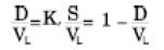
1. The capital structure is constant:
I begin with the most fundamental equations:
Let EBITDAi be earnings before interests, taxes, depreciation and amortization for period i, Dep= Depreciation, D=Debt, kD=Cost of Debt, T=Tax rate, ΔNwc= Increment in net working capital and ΔFA=Increment in fixed assets.
Then ECFi = (EBITDAi - Depi - DikD)(1-T)+ Depi + gDi - ΔNwci - ΔFAi is the equity cash flow and FCFi = (EBITDAi - Depi)(1-T) + Depi - ΔNwci - ΔFAi is the free cash flow. The relationship between both is FCFi = ECFi+Di kD (1 - T) - gDi
To simplify things I suppose ΔNwci = kwEBITDAi; ΔFAi = kFAEBITDAi. The free cash flow becomes FCFi = (EBITDAi)(1 - T - kw - kFA) + TDepi
Under this approach Depi also becomes proportional to EBITDAi:
Let Dr=1/y (y=years for full depreciation), suppose Dr is constant over the years (for 10 years depreciation, Dr=10%); TGA= Total gross assets, FDA= Fully depreciated assets, then: Depi=[TGAi-1-FDAi-1]Dr
For i>y,
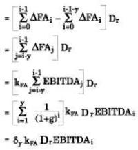
Where δy 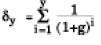
k0 is the discount rate for the firm assets, under a cero leverage policy (more on this rate follows). When leverage is greater than cero, the firm value results from the combined effects on the cash flows to debt holders and shareholders. As per assumption 1, the debt increases at the same rate (g) that the cash flows, then Di+1=Di(1+g).1
The cash flow to the debt holders is: DCFi = -gDi + kDDi
Then cash flow to the investors, shareholders (ECF) and debt holders (DCF) is:
CF(VL)i = ECFi + DCFi = (EBITDAi - Depi - Di kD) (1-T)+ Depi + gDi - ΔNwci - ΔFAi -gDi + kDDi = FCFi + kDDiT2
CF(VL) = FCF1 + kDD0T, discounting the flows at the appropriate3 rates yields:
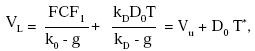 Where
Where 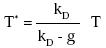
Fernández (2003) arrives to a different expression for the Tax Shield:  He avoids cash flows and employs valuation equi valences.
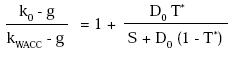
kD is the interest rate for the firm debt, here I assume that this rate is the same rate that the debt holders are receiving. Under certain conditions these rates differ. The convergence condition is more severe, it requires that g < kD.4 The second term D0T*, is known as the tax shield, except that the effective tax rate is higher, yielding a higher firm value.
]]> A market balance at t=0 follows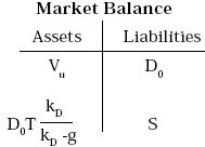
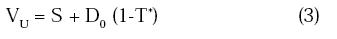
Solving the accounting identity for VU, we find an additional definition for the unlevered firm:
kS, the equity cost for the levered firm
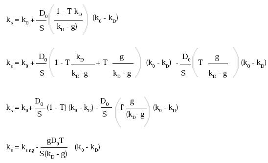
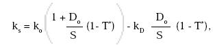
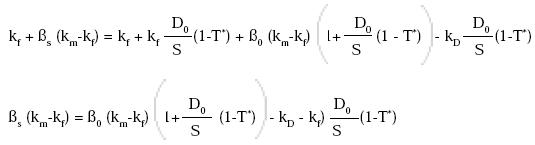
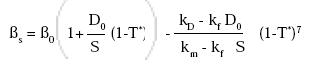
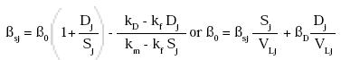
Now we have enough tools to find kS. The cash flows produced by the assets and by the liabilities should be the same, then it must be that VU k0 + D0 T* kD = Sks + D0kD,5 replacing VU with equation 3 and solving for kS, we obtain:
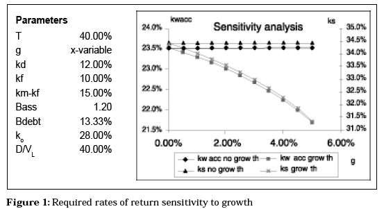
The above result is the familiar definition of kS, modified by the new effective tax rate. Interestingly, increasing flows reduce the required rate of return for the shareholders (Figure 1), when k0 > kD. We can also express this result as a combination of the standard equity cost with no growth kS ng and the growth effect.
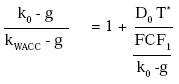
As long as k0 > kD, the growth effect is negative. Lets proceed to check if under these conditions continue to hold another basic financial result: That discounting the unlevered flows at the weighted average cost of capital yields the same number that discounting the unlevered flows at the required rate of return for the firm assets plus the increased tax shield. To do this, is enough to find what definition of kWACC solves the following equality:
]]>
First multiply both sides of the equality by  the result is
The last result is the same (by equation 1) that 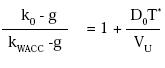
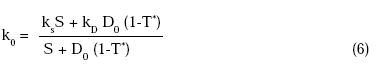
Replacing VU by equation 3 yields
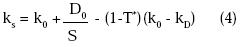
Solving equation 4 for k0 results in
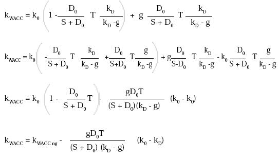
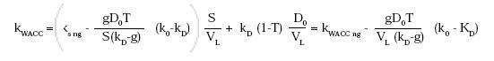
We use this result in the equation 5 and solve for kWACC:
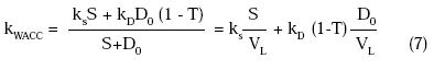
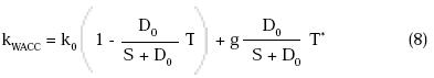
The previous equation shows that the effects of the constant growth are two fold. First, is a decreasing effect caused by the interaction of k0 and T* and, second, an increasing effect through the interaction of g and T*. Under no growth we have 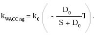 With that in mind, modifying equation 8 yields6
As we saw before, under normal conditions (k 0 > k D) the decreasing effect dominates (Figure 1).
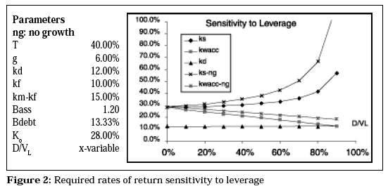
The effects of leverage on the different required rates of return (Figure 2) shows how the kWACC decreases at a higher rate with constant growth and the ks increases at a lower rate. Again the benefits of growth are significant.
It is noteworthy to understand that only with the corrections here developed continue to hold the equality
MODIFIED BETA CALCULATIONS
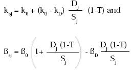
The fundamental equation of CAPM permit us to find some additional equivalences. By the CAPM we have ks = kf + βs (km - kf)and ko = kf + βo (km - kf), where the meaning of the different terms correspond to the usual ones. Rewriting equation 4 yields:
 combining it with the former CAPM equations produces:
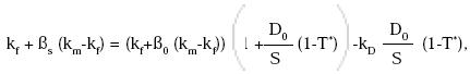
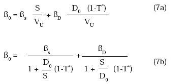
reordering terms gives the following result:
7Most of the time the second term of this equation is ignored, the unique occasion when this practice is right is for kD=kF, which implies that βD=0.
]]> By CAMP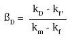 Then
Then 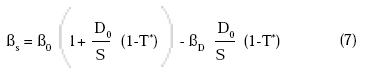
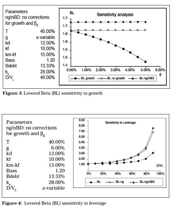
Or
The previous equations also shows that we have to reformulate our beta calculations when considering constant growth. Figures 3 and 4 illustrate the consequences of ignoring the corrections here contemplated. Note how the practice of ignoring βD increases the gap.
OPERATIONAL REMARKS
The next paragraphs explore different approaches that use the concepts developed above. In particular they cover:
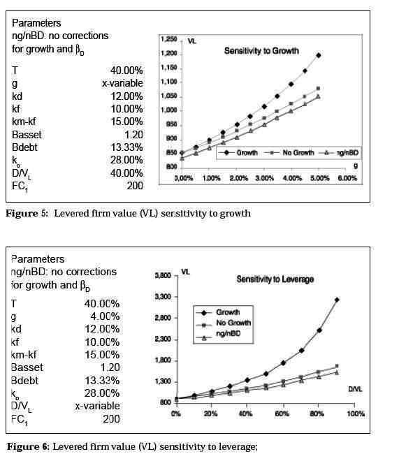
Here I performed sensitivity analysis to growth rates and leverage similar to those performed for the required rates of return and betas. Not surprisingly the consequences of ignoring the adjustments lead to undervaluation, that increases with growth and leverage.
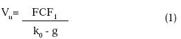
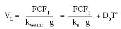
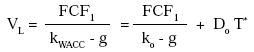
The valuation formula we use is 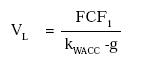 an infinite growing perpetuity.
Under this scenario the basic assumptions does not hold and we cannot use a unique kWACC to discount the cash flows, because it is changing each period. The only option left is to estimate the tax shield directly. If the debt is increasing but a different rate (g1), it is still possible to use the same technique. For the estimation of the tax shield in the general case see the valuation example.
]]> Market BetasThe use of market betas is implicitly explained in the previous section. Here the lesson it is do not forget the correction for βD or its proxy (kD-kf)/(km-kf). Measuring β0 correctly implies to adjust for the cost of debt.
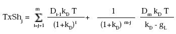
How we implement a working model of these developments. The answer is that real calculations should use expressions that very each period; then the firm value needs to be solved backwards. Suppose the estimations of FC cover period 1 to period m, after that a constant growth gL is expected.8 For any period j≤m holds
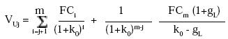
The Tax Shield is
VLj = VUj + TxShj = Sj + Dj, which gives us an expression for the unlevered firm for the period j:
VUj = Sj + Dj - TxShj
The cash flows produced by the assets and the liabilities should be the same, then
]]> Sj ksj + Dj kD = VUjk0 + TxShjkD = (Sj+Dj - TxShj) k0 + TxShj kDEven though we suppose that kD, T and K0 are constant over time, this is not required and a subindex can be incorporated for a complete generalization. The assumption 1 (A constant leverage) is also relaxed for periods less than m (which applies to m+1 cash flows). Solving for ksj yields
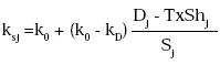
Now for each period holds:
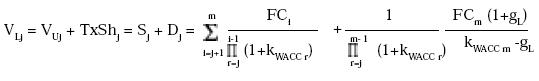
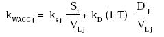
Again the expression for kWACCj is
Each period has a set of simultaneous equations; implementing those equations in a spreadsheet produces circularities, which are solved through iterations.9
The implementation, which is illustrated in Table 1, begins when the forecasted flows begin to growth at a constant rate. Here holds all the equations we deduced in the above paragraphs:10
]]>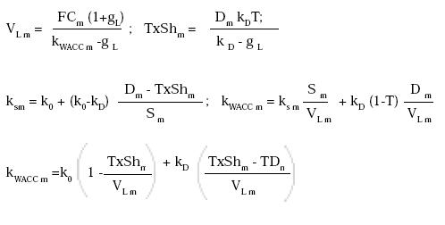
To solve the equations system, some inputs are required:
FCm, T, kD,k0,gL and either Dm or the target leverage Dm/Sm.
Now we go backwards to solve the equations for the period m-1:
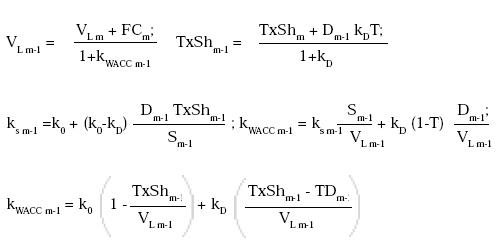
The same formulas apply for the periods m-2 to 0. The algorithm stops when we reach the period 0.
Having sketched the approach, the numerical example is worked.
The Table 1 shows how this technique produces similar valuations (period by period): (1) through the direct discount of the free cash flows with kWACCj; and (2) through the discount of free cash flows with k0 plus the Tax Shield (The Adjusted Present Value proposed by Myers). The result holds for kD, k0 and T not constant.
With this methodology the effect on ks of the growing perpetuity only affects the period m. Given that the terminal value is not a negligible part of the firm value, the economic effects of this correction continue to be significant.
Finally, following the same procedure outlined before, we have:
]]>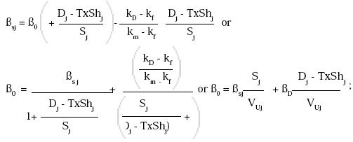 for the operational model we develop.
 Another history results if we accept the correction to the M&M model proposed by Harris and Pringle (1985). For them the tax shield bears the assets risk (k0) not the debt risk. In this universe ksj = k0 + (k0 - kD) Dj Sj and the effect of growth is not explicitly incorporated to the expression of ks j, here the effect is indirect and only present when the leverage is not constant (or the amount of debt is constant). As expected the valuation results are lower and the difference increases with the distance between k0 and kD. The corresponding expressions for the betas are:
The Fernandez (2003) model also doesn´t incorporates the effect of growth in their cost of capital or beta, the equations are:
He critics M&M (1963) and Myers (1974) on the grounds of ks<k0 for some values of g, but all the models growing perpetuities (including Fernandez) depend critically this measure. question if expected growth should reduce cost capital is important, here we differentiate operational risk and its required return from growth. Myers (1974) approach correct, capital: Are investors more prone to invest in firms with high growth, other things equal (specially assets risk)? answer yes (which sounds reasonable) empirical data confirm it.
CONCLUSIONS
The equations have worked present a coherent system that preserves under conditions equality VL = Vu + TS. They also show higher continuing constant produces lower equity. conclusion true, Among working same business (similar k0), those equity risk. On side, corrections by Harris Pringle (1985) or Fernandez (2003) holds, the cost of equity shouldn´t be affected As it has been stated before, tax shield becomes risky when leverage increases firm size does not isolate market adjustments. The tax shield also depends of the firm´s ability collect it, even after losses.
]]> A empirical test seems appropriate; after all, corporations always forecast growth. That test is feasible. Firms with higher growth should have a lower kWACC. Measuring kWACC does not depend of how ks is stated. We can estimate ks through its CAPM definition ks = kf + βs(km - kf). The cost of debt does not change and can be ignored. Controlling for industry and size should be enough to see how the predictions deals with reality.FOOTNOTES
1. To check this assertion is enough to note that VLi+1=VLi(1+g), without FCFi+1. Given that the debt proportion is constant, it follows that D grows at the same rate. Interest payments are due at the end of period.
2. Under Fernandez (2003) approach:
Tax Shield=TxU - TxL = EBITDA(1-δykFADr)T- [EBITDA(1-δykFADr) + kDD]T = kDDT.
The result is the same. The key difference is that for Fernandez TxU and TxL have different risk and should be discounted independently, under the assumptions of this paper that doesnt hold.
3. As I said, the discount rate for the tax shield is an unsolved issue on valuation, here I assume that this rate is the debt rate as Myers (1974).
4. It is not difficult to conceive firms with g > kD, the only attenuant is that it is difficult to maintain indefinite growth rates higher than the cost of debt.
5. The result is the same if the equation is written for increasing flows VU (k0-g)+D0T* (kD-g) = S(ks-g)+D0(kD-g).
6. A simpler approach is to note that.
]]>
8. The idea here is to present a methodology where the calculations are applied for the different periods.
9. To activate that feature in Excel go to Tools, choose Options, then Calculations; check in the Iterations box. See Velez and Tham (2001).
10. Implicitly we went back to assumption 1 (constant leverage).
BIBLIOGRAPHY
Fernández, Pablo. 2004. The value of tax shields is NOT equal to the present value of tax shields. Journal of Financial Economics, 73(1). [ Links ]
Harris, Robert S. and John J. Pringle. 1985. Risk-adjusted discount ratesextensions from the average-risk case. The Journal of Financial Research 8, 237-244. [ Links ]
Modigliani, Merton and Merton Miler. 1958. The cost of capital, corporation finance and the theory of investment. American Economic Review 48, 261- 297. [ Links ]
Modigliani, Merton and Merton Miler. 1963. Corporate income taxes and the cost of capital: a correction. American Economic Review 48, 261-297. [ Links ]
Myers, Stewart C. 1974. Interactions of corporate financing qand investment decision-Implications for capital budgeting. The Journal of Finance 29, 1-25. [ Links ]
Ross, Stephen A., Randolph W. Westerfield and Jeffery Jaffe. 1999. Corporate Finance, 5th Edition. Boston: Irwin McGraw-Hill [ Links ] ]]>