CARLOS EDUARDO ORTIZ-YUSTY
VIVIAN PÁEZ
FERNANDO A. ZAPATA

Departamento de Biología, Universidad del Valle, Santiago de Cali, Colombia.carlosyu1286@gmail.com

Instituto de Biología, Universidad de Antioquia, Medellín, Colombia.vivianpaez1@gmail.com

ABSTRACT

Our objective was to explore the spatial distribution patterns of amphibian species richness in Antioquia, as model for the tropical Andes, and determine how annual mean temperature, annual precipitation, and elevation range influence it; and to briefly compare local and global regression models for estimating the relation between environmental variables and species richness. Distribution maps for 223 amphibian species and environmental variables were generalized onto grid maps of 752 blocks each covering the entire of Antioquia. We explored the relationship between species richness and environment using two global regression models (the Ordinary Least Squares "OLS" and Generalized Linear Squares "GLS" models) and one local model (the Geographically Weighted Regression "GWR" model). We found a significant relationship between species richness and environmental variables (GLS r²: 0.869; GRW r²: 0.929). The GLS model efficiently incorporated the spatial autocorrelation effect and handled spatial dependence in the regression error terms while the GWR model showed the best fit (r²) and balance between number of parameters and fit (AICc). GWR parameters show wide variation within the study area, indicating that relationship between species richness and climate is spatially complex. Temperature was the most important variable in the GLS and GWR models, and altitude range the least significant. The strong relationship between environment and amphibian richness is possibly due to life history traits of amphibians, such as ectothermy and water dependency to complete the life cycle.

Keywords: Amphibians, spatial pattern of species richness, spatial regression models, environmental variation, macroecology.

RESUMEN

Nuestro objetivo fue el de explorar el patrón de distribución espacial de la riqueza de especies de anfibios en el departamento de Antioquia, Colombia y determinar cómo la temperatura anual, la precipitación anual y la heterogeneidad altitudinal afecta este patrón, como modelo para los Andes tropicales. Para ello, delineamos mapas de distribución de 223 especies de anfibios que habitan en Antioquia y junto a mapas de las variables ambientales  se generalizaron en cuadrículas de 752 celdas que cubrían todo del departamento. La relación entre riqueza de especies y ambiente fue determinada utilizando dos modelos globales de regresión (modelo OLS y GLS) y un modelo local (modelo GWR). Se encontró una relación significativa entre la riqueza de especies y el clima (GLS r²: 0.869; GRW r²: 0.929), donde la temperatura fue la variable más importante, mientras que la heterogeneidad altitudinal no fue significativa. El modelo GLS mostró mayor eficiencia en incorporar  el efecto de la autocorrelación espacial en los términos del error, mientras que el modelo GWR mostró un ajuste mayor (r²) y mejor balance entre número de parámetros y ajuste (AICc). Los coeficientes de regresión en el modelo WGR mostraron una gran variación a lo largo del área de estudio, indicando que la relación entre la riqueza de especies y las variables climáticas es espacialmente compleja. La fuerte relación entre ambiente y riqueza de especies de anfibios puede atribuirse a las características de historia de vida como la condición de ectotermos y la dependencia de humedad para la reproducción.

Palabras clave: Anfibios, Patrón espacial de riqueza de especies, modelos de regresión espacial, variación ambiental, macroecología.

Recibido: 21/08/2011
Aceptado: 04/04/2013

INTRODUCTION

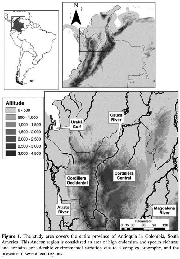
Biological and ecological phenomena that vary spatially are often spatially autocorrelated (i.e., nearby sampling units tend to have similar values for a variable, and this similarity decreases as distance increases). This represents an issue in statistical analyses, because the data might not be totally independent (Legendre 1993, Diniz-Filho, et al. 2008) making hypothesis testing overly liberal because the number of sample units overestimates the true number of degrees of freedom, increasing the probability of making Type I errors (H-Acevedo & David 2003). Thus, the omission of spatial dependence in statistical analyses may lead to misinterpretation of the results, biased parameter estimates, and false detection of significant relations (Legendre 1993). Another issue is the change in coefficient estimates in regression models that do not correct for the spatial component, compared to those that do, which affects the ability to assess the significance of predictor variables (Lennon, et al. 2000).

Many methods of spatial analysis have been used for decades in the geostatistical literature (Besag 1974), and their application in ecology and species distribution research has been growing (e.g., Jetz & Rahbek 2002, Diniz-Filho, et al. 2003, Wang, et al. 2005, Kissling & Gudrun 2008). Most applications of regression models in ecology involving spatial data have been restricted to the incorporation of spatial dependence, but few studies have tested model specifications, their performance and potential for accounting for spatial autocorrelation, or the accuracy of parameter estimates (Kissling & Gudrun 2008). There are many studies focused on quantifying the relationship between climate and distributional patterns of species richness at regional levels using birds and mammals (Badgley & Fox 2000, Baquero & Telleria 2001, García-Trejo & Navarro 2004), while relatively few have focused on ectoterms like fishes or amphibians. Studies exploring the relationship between environmental gradients and amphibian species richness from a biogeographical and macroecological approach have mainly been conducted in North America, Europe and Australia (e.g., Bock & Smith 1982, Fraser 1998, Boone & Krohn 2000, Buckley & Jetz 2007). Those that include South America generally are conducted at a continental scale with low resolution (i.e., (Cassemiro, et al. 2007).

Colombia offers a great opportunity to study patterns of diversity in tropical Andean amphibians. It is currently considered one of the countries with the greatest amphibian richness, with 720 species (according to the IUCN), thanks to its geographical location and diverse topographic and climatic characteristics that combine to produce varied habitats and microhabitats (Rueda Almonacid, et al. 2004).  The main objectives of this study were to document the spatial distribution patterns of amphibian species richness in the north Andean province of Antioquia – Colombia, as a model for Andean amphibians. Additionaly, determine the degree of geographic variation explained by annual mean temperature, annual precipitation, and elevation range, as well as to compare the performance of global models with respect to a local model for estimating the relationship between species richness and these environmental variables.

MATERIALS AND METHODS

The study area covered the entire province of Antioquia, located in the Andean region of northwestern Colombia (Figure 1). It is considered an area of high endemism and species richness (Lynch, et al. 1997). Although Antioquia is a political, rather than biogeographical or ecological unit, its territory contains considerable environmental variation due to its size, a complex orography, and the presence of several eco-regions. Antioquia has an area of 62 150 km², which extends from the Atrato River on the west to the Magdalena River on the east, with a coastline of 240 km on the Gulf of Urabá on the Caribbean coast and two parallel mountain ranges (Cordillera Occidental and Cordillera Oriental) that bisect the department, attaining elevations up to 4 000 m (Figure 1).

Antioquia contains approximately 30% of the known amphibian species of Colombia and despite problems of incomplete sampling, there is sufficient information available in the literature, databases, and museum catalogues to permit construction of species richness distribution maps. Such maps may be used as first approximations to identify patterns that may help to understand the processes underlying the generation of particular distributions of species richness and aid in locating protected areas or biological corridors or guiding management decisions for this vulnerable taxon (Scott, et al. 1993).

Response variable – Species Richness

We used the distribution maps for 223 amphibian species known to breed in Antioquia (207 anurans, 8 caecilians and 8 salamanders) from the Global Amphibian Assessment (http://www.globalamphibians.org), and the altitudinal distribution information from the online reference of the American Museum of Natural History (http://research.amnh.org/herpetology/amphibia/). Some of the IUCN maps are inaccurate or have a low resolution in the study area, so we supplemented these maps with potential distributions. We used Maxent 3.3.3e software (Phillips, et al. 2006) to run distribution models for the 223 amphibian species for which we had 8,573 single geographic records from the Museo de Herpetología Universidad de Antioquia (MHUA) and another 13 biological collections (covering specimens collected from 1921 to 2007; Table 1), under the "auto-features" mode as suggested by Phillips & Dudik (2008) and including 19 environmental variables obtained from the Worldclim online database (Hijmans, et al. 2005).

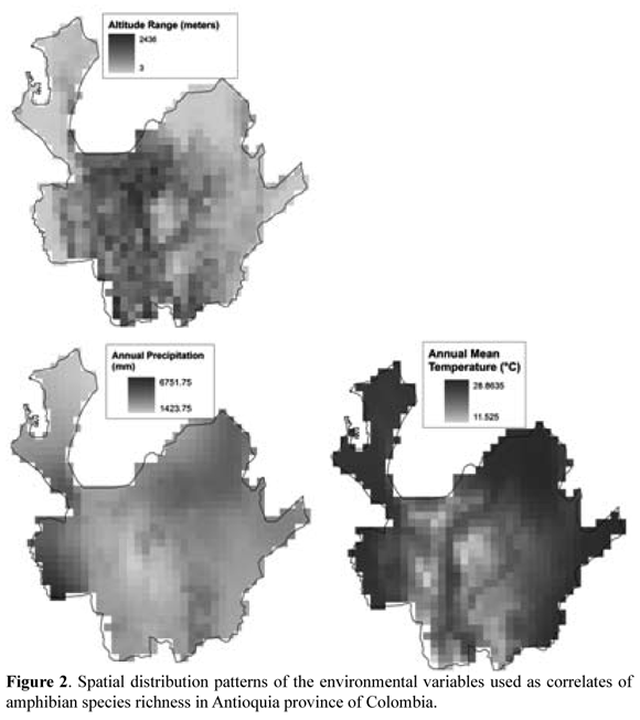
Each of these distribution ranges was generalized into grids with 752 cells of 80 km² each, covering the entire province of Antioquia. The presence of each species in a cell was determined by the overlap of the smooth-line over at least 50% of the cell.  The species richness for each block was calculated by counting the number of species present (Boone & Krohn 2000, Diniz-Filho, et al. 2008). Large-scale approaches to building species geographical range maps require two important assumptions: the spatial patterns do not change over time and species distributions are continuous across the mapped range (Gotelli & Graves 1996). However, no species has a continuous distribution, regardless of the scale (small, medium or large) at which it is considered, and a representation of a distribution as a polygon or map is a simplification; however, this does not invalidate these analyses since the resulting distributions still convey real preferences and climatic limits for a species (Gotelli & Graves 1996).

Independent variables – Environmental variables

We used annual mean temperature, annual precipitation, and elevation range as predictor variables. These variables have commonly been related to spatial variation in species richness (Schall & Pianka 1978, Boone & Krohn 2000, Diniz-Filho, et al. 2004). Environmental variables were extracted from the online database "Worldclim 1.4" (http://www.worldclim.org/) and adjusted to the same spatial resolution as the species richness data (Figure 2). Elevation range corresponds to the difference between maximum and minimum elevation in each cell, as a proxy of environmental heterogeneity. This particular environmental data set was selected because it includes data from 1950 to 2000 (Hijmans, et al. 2005) and thus matches well the period of collection of museum specimens.

Regression Analysis

Three methods were used to examine the relationship between species richness and environmental variables: two global models, the Ordinary Least Squares (OLS) and Generalized Least Squares (GLS) models, and a local model, the Geographically Weighted Regression (GWR) model. Both global approaches estimate a single parameter or coefficient for each predictor variable that applies to the entire study area (i.e., consider the landscape as one unit), while the local method allows parameter values to vary continuously in geographical space (i.e., defines parameters for each location in the landscape under study).

The assumption of global regression methods (OLS, GLS) is that the relationship under study is constant (i.e., stationarity), and therefore the estimated parameters remain constant in space, which is not always true. In contrast, the GWR technique allows local influences, leaving the parameters free to vary spatially and fit more appropriately (Fotheringham, et al. 2002). Although the technique does not allow extrapolation beyond the region where the model has been applied, by allowing the parameters to vary locally within the study area a more accurate and appropriate basis for descriptive and predictive purposes is achieved (Foody 2003).

The high number of species with small geographic ranges and the geographic complexity of study area could produce variations in the relationship among richness and climate in different regions of Antioquia. A global model with a single best predictor will be the best choice for extrapolation or to know the general relation between variables under study. However, to determinate how relationships between predictor and response variables varies in the space, a locally weighted model can help to reveal spatial variation in the empirical relationships between variables that otherwise might be ignored in the analysis.

The OLS model is the standard linear regression and can been viewed as:

Where Y is a vector (n x 1) with a response variable, X is a matrix of predictive variables (n x (p + 1)), β is a vector of estimated parameters or constants ((p + 1) x1) and ε is the vector containing the error terms (n x 1). The OLS model requires the residuals to be independent (Jobson 1991). Otherwise, the estimated parameters of the model may be imprecise while confidence intervals may be underestimated, which increases Type I error (Legendre 1993). This happens when there is spatial autocorrelation. Thus, the OLS model is not recommended in studies that include spatially distributed variables (Diniz-Filho et al. 2003). For this reason, this regression analysis was used for comparative purposes only.

The GLS is derived from standard regression, but differs in the incorporation of the spatial structure directly into the residuals with the aim of estimating the "true" regression coefficients, modifying the way vector β is estimated (Dormann, et al. 2007). This model has been proposed as one of the most efficient ways to obtain the regression coefficients in the presence of autocorrelation (Jobson 1991). The vector β is now estimated as follows:

β = (X^T C^-1 X)^-1 X^T C^-1 y

Where X and Y have the same notation as in Equation 1, and C is a square matrix (n x n) describing the covariance between pairs of residual values of the model. In this case, the values of the covariance matrix C were modeled using a function derived from a semi-variogram adjusted to a spherical model, calculated as:

y(d) = C₀ + C₁ (1.5 (d/a) - 0.5 (d/a)³) si d <= a; y(d) = C si d > a

Where y is the semivariance, C is the covariance, d is the distance between pairs of localities, C₀ is the variance unexplained by the model, C₁ is the maximum semi-variance between localities (and must match the population variance), and a is the distance where the variance ceases to increase (Jobson 1991).

The GWR model is a recent refinement of the standard regression methods that deals explicitly with spatial nonstationarity of the empirical relationships (Fotheringham et al. 2002). This technique provides a weight for information that is locally associated, allowing the regression model parameters to vary in space. From the global OLS model, the GWR model can be viewed as:

Y = Xβ(µ, v) + ε

Where (µ, v) denotes the coordinates of the samples in space. The regression parameters are estimated as follows:

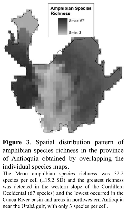
Where β(µ, v), represents an estimate of β; W(µ, v) is the weight matrix and X the matrix of independent variables, determined for this case with the "Bi-square" function:

W _ij = (1 - (d_ij/b)²)²

Where W _ij, is the weight of a specific point j in space where the data are observed at any point i in space where the parameters are estimated; d_ijis the distance between points i and j; and b the bandwidth, obtained with the Akaike information criterion optimization module include in SAM 3.0 (Rangel, et al. 2006).

The degree of spatial autocorrelation in the predictor and response variables and regression residuals were estimated by constructing omnidirectional correlograms based on Moran's I coefficient, using the statistical program SAM 3.0 (Rangel et al. 2006). Collinearity was estimated  using a correlation matrix among predictor variables and the Condition Number (CN), which according to Lazaridis (2007) is CN= (max/min)-1/2, where max and min refer to the highest and lowest correlation value extracted from the correlation matrix between predictor variables, respectively. With a CN > 5, the model is likely affected by multicollinearity, values between 2 and 5 denote the presence of multicollinearity that probably does not greatly affect the model, and values of less than 2 clearly indicate multicollinearity is not an issue.

Regression Model Evaluation

Selection procedures that allow the identification of the best model or set of best models to describe patterns under study are lacking in most ecological studies where data are autocorrelated (Johnson & Omland 2004, Kissling & Gudrun 2008). Here we apply three selection criteria proposed by Kissling & Kudrun (2008) to evaluate the performance of these regression models, based on the existence of three ideal characteristics that a model must satisfy in the presence of autocorrelated data:  1) eliminate the autocorrelation of the residuals to avoid increasing the probability of making Type I errors, 2) obtain a maximum fit to make more accurate descriptions and predictions, and 3) achieve a good balance between number of parameter and fit. Those criteria were: the Minimum Residual Spatial Autocorrelation (minRSA), computed by adding the value of Moran's I coefficient of the 19 distance classes obtained directly from the residual correlograms of each model; the maximum model fit (r²) and the Akaike Information Criterion (AICc).

RESULTS

Amphibian richness

Mean amphibian species richness per cell was 32.2 (±15.2 SD). The greatest species richness was detected in the western slope of the Cordillera Occidental, in the biogeographic Chocó region, that contains up to 67 species per cell; and the lowest species richness occurred in the Cauca River basin (that runs between the Cordillera Central and Cordillera Occidental of the Andes mountains) and areas in northwestern Antioquia near the Urabá Gulf, with only 3 species per cell (Figure 3).

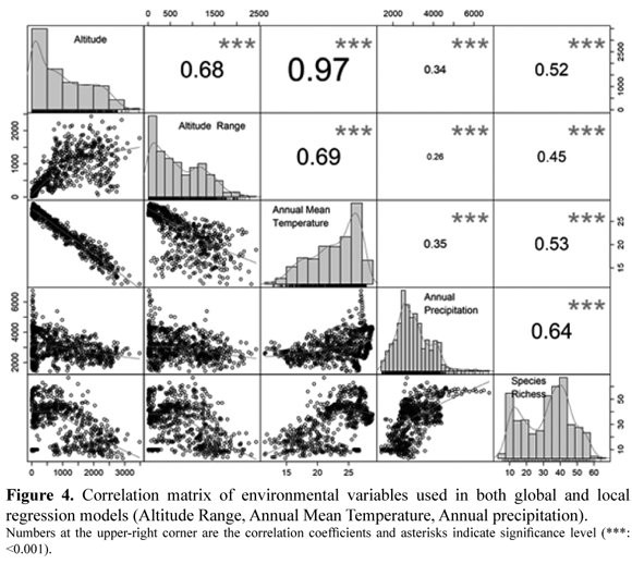
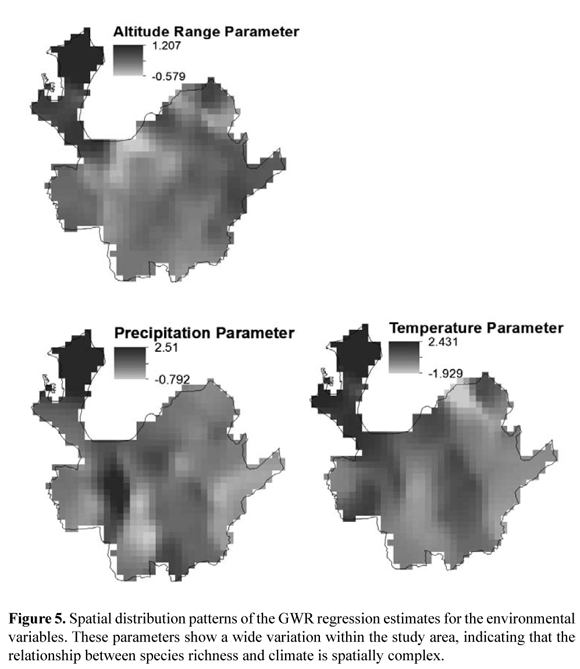
Regression Analysis

Correlograms obtained with Moran's I coefficient for species richness and the environmental variables showed positive autocorrelation (p< 0.05) in all cases for the first distance classes, with linear decreases in autocorrelation (covariance) as distances increased. We only detected a relatively high correlation between annual mean temperature and altitude range (r= 0.69; Figure 4). Additionally we found a low condition number (CN= 2.503), both indicating presence of collinearity in the models, but it was low and possibly did not strongly affect the estimated parameters (Lazaridis 2007).

With both global (OLS and GLS) and local (GWR) regression models, significant relationships between species richness and the environmental variables were obtained; however, the amount of variation explained (r²) was different:  the OLS model explained 53% of the variation in species richness based upon the environmental variables, while the GLS model explained 86% and the GWR model explained 92.9% (Table 2). The models also differed in the relative contribution (standard coefficients) and significance of each variable considered. In the OLS model, all variables contributed significantly (p < 0.001) to accounting for the variation in amphibian species richness. The most important variables were annual precipitation, followed by annual mean temperature with both showing a positive association with amphibian species richness (Table 2). Altitude range was the variable that contributed least and also presented a negative association with species richness. In the GLS model, altitude range was not significant (p = 0.175) and annual mean temperature was the variable that explained the most variance in the model (p < 0.001). Both annual mean temperature and annual precipitation presented positive slopes (Table 2).

With the local (GWR) regression model, we found that altitude range exhibited a negative relation with species richness in most of Antioquia, or presented values near zero, with the variable exhibiting a positive relationship only in the northwest. Annual mean temperature showed the greatest spatial variation in the local estimated coefficients, with a positive relationship in the northwest, on the eastern flank of the Cordillera Central and western flank of the Cordillera Occidental. Annual precipitation also showed a negative relationship throughout most of the department and was positive in the western flank of the Cordillera Central and in the northwest (Figure 5). According to the median obtained for local regression coefficients of each predictor, annual mean temperature was the variable that most contributed to the regression model and also presented the greatest range of variation. In contrast, the local coefficients of altitude range presented a median near zero and the smallest range of variation. As a result, this variable was of lesser importance in the regression analysis (Table 2).

Regression Model Evaluation

According to the selected evaluation criteria (minimum residual autocorrelation, r² and AICc), the GLS and GWR models performed better than the OLS model (Table 2). The GWR model presented the best fit, accounting for 93% of the variation in species richness. This model also had the lowest AICc score, which indicates that the model had a better balance between number of parameters and amount of variance explained. The GLS model incorporated and managed the spatial dependence of the input variables better than the other models since the spatial autocorrelation was eliminated almost entirely from the residuals (Table 2)

We found a high correlation between amphibian species richness and environmental variation, with temperature being the most important variable, followed by precipitation. Elevational range showed the lowest correlation. Previous studies also have noted that variance in elevation has little relation to amphibian richness. For example, Owen (1989) found that the variance in elevation explained less than 15% of the variation in species richness in Texas. Kiester (1971) also mentioned a similar pattern when he compared continental maps of amphibian and reptile richness with the mammal maps of Simpson (1964), and noted that mammal richness was more closely related to topography than amphibian and reptile richness. Owen (1989) suggested that amphibians are less tolerant to the extreme climates of highlands than groups such as mammals, and that the differences between mammals and amphibians in the relationship between richness and environmental variables was due to differences in their average body sizes.

The correlogram profiles obtained with the environmental variables and species richness (positive autocorrelation at short distances coupled with negative autocorrelation at large distances) suggest that there is spatial structure only at small scales, and it corresponds to one of the three profile types usually found in ecological data, which can be interpreted as a linear gradient of the variables studied at broad scales (Diniz-Filho, et al. 2003). There is a relationship between topography and variation in amphibian species richness mediated by the climatic variation caused by the influence of the Andes mountain ranges in the province. The temperature of the troposphere decreases at a relatively constant rate of 7° C with an increase of 1 km in altitude, so the mountains can increase the amount of precipitation, change the movements of storms and cause uplift of air masses that increase moisture levels (Hobbs & Wallace 1977). Additionally, topography also may cause the amount of sunlight that is projected onto an area to vary, which also has been associated with species richness (Currie 1991).

The climatic variables considered here showed significant positive correlations with species richness. However, negative correlation zones also were observed with the GWR model.  Annual total precipitation was one of the most important environmental parameters for explaining amphibian richness variation at intermediate and broad spatial scales. Boone & Kronh (2000) found that precipitation was the variable most correlated with species richness of salamanders, frogs and turtles in the state of Maine (USA). This was consistent with Kiester (1971), who found that amphibian species density was strongly correlated with annual rainfall on a continental scale.

In this study, temperature had a higher relative importance in regression models due to amphibian's sensibility to temperature changes. Additionally, their distributional ranges and behavioral patterns may be largely limited by this parameter (Zug, et al. 2001). It has been reported that ambient temperature regulates physiological and metabolic function of anurans (Duellman & Trueb 1994), and their activity temperature can also be predicted from ambient temperature (Navas 2002). Precipitation was also associated with amphibian richness, but had a secondary role in comparison with temperature in our analysis. Most amphibian species are strongly associated with humid zones for breeding and completing their life cycle. Thus, humidity is an important factor determining their distribution; further, their thermal physiology is also strongly coupled with ambient moisture level (Pearson & Bradford 1976). However, water availability possibly is not an issue in most of the tropical Andes, since there are several permanent sources of running and still water, such as rivers and streams (Navas 2002), ensuring a vast quantity of breeding sites and an adequate environment, supplying good conditions for gas exchange and preventing desiccation.

The model fit (r²) and performance (AIC) of the GWR model was superior to the OLS and GLS models.  This suggest that the relationship among species richness and the environmental variables is not constant in space (Fotheringham, et al. 2002). The GWR parameter variation shows a very complex relationship between climate and species richness across space and suggests an interplay with other factors like biogeographical history or speciation/extinction patterns. The spatial patterns revealed by the parameters of the GWR model illustrate a potential danger of using a single estimate derived from global models. Estimates calculated with global models fail to represent the relationship between species richness and environmental variables in most areas of the region and may have little descriptive and predictive value.

We found a strong relationship between temperature and precipitation with amphibian species richness, which would be consistent with the energy hypothesis and possibly the determination by physiological factors is the primary mechanism (Navas 2002, 2006). Both temperature and precipitation have been regarded as strong factors determining amphibian richness in the world (Boone & Krohn 2000, Buckley & Jetz 2007), but in the tropical Andes the high availability of water sources makes precipitation a less important factor than temperature (Navas 2002, 2006). However, this result may not be definitive, since it has been showed that the spatial resolution at which analyses are performed affects the relative importance of different environmental factors in the models (Rahbek & Graves 2001, Graham & Hijmans 2006).

ACKNOWLEDGMENTS

We are grateful to many people from the Grupo Herpetológico de Antioquia (GHA) who helped in the collection and data cleaning of museum records, including Juan Pablo Hurtado and Natalia Silva. We thank Adriana Restrepo, Brian Bock, Juan Manuel Daza, Julián Velasco and Christopher Parkinson for comments on the manuscript, and Juliana Jaramillo for her help in the translation of this document. We finally thank two anonymous referees who provided very helpful and insightful comments on the manuscript.

LITERATURE CITED

1. BADGLEY, C. & D.L. FOX. 2000. Ecological biogeography of North American mammals: Species density and ecological structure in relation to environmental gradients. Journal of Biogeography 27: 1437-1467         [ Links ]

2. BAQUERO, R.A. & J.L. TELLERIA. 2001. Species richness, rarity and endemicity of European mammals: a biogeographical approach. Biodiversity and Conservation 10: 29-44        [ Links ]

3. BESAG, J. 1974. Spatial interaction and the statistical analysis of lattice systems. Journal of the Royal Statistical Society. Series B (Methodological) 32: 192-236        [ Links ]

4. BOCK, C.E. & H.M. SMITH. 1982. Biogeography of North American amphibians: A numerical analysis. Transactions of the Kansas Academy of Science (1903-) 85: 177-186         [ Links ]

5. BOONE, R.B. & W.B. KROHN. 2000. Partitioning sources of variation in vertebrate species richness. Journal of Biogeography 27: 457-470         [ Links ]

6. BUCKLEY, L.B. & W. JETZ. 2007. Environmental and historical constraints on global patterns of amphibian richness. Proceedings of the Royal Society B: Biological Sciences 274: 1167-1173        [ Links ]

7. CASSEMIRO, F.A.D.S., B. BRUNO DE SOUZA, L.V.B.R. THIAGO FERNANDO & D.-F. JOSÉ ALEXANDRE FELIZOLA. 2007. Non-stationarity, diversity gradients and the metabolic theory of ecology. Global Ecology and Biogeography 16: 820-822         [ Links ]

8. CURRIE, D.J. 1991. Energy and large-scale patterns of animal-and plant-species richness. American Naturalist 137: 27        [ Links ]

9. DINIZ-FILHO, J.A.F., L.M. BINI & B.A. HAWKINS. 2003. Spatial autocorrelation and red herrings in geographical ecology. Global Ecology and Biogeography 12: 53-64        [ Links ]

10. DINIZ-FILHO, J.A.F., L.M. BINI, C.M. VIEIRA, M.C. DE SOUZA, R.P. BASTOS, D. BRANDAO & L.G. OLIVEIRA. 2004. Spatial patterns in species richness and priority areas for conservation of anurans in the Cerrado region, Central Brazil. Amphibia-Reptilia 25: 63-75        [ Links ]

11. DINIZ-FILHO, J.A.F., T.F.L.V.B. RANGEL & L.M. BINI. 2008. Model selection and information theory in geographical ecology. Global Ecology and Biogeography 17: 479-488        [ Links ]

12. DORMANN, C., J. MCPHERSON, M. ARAÚJO, R. BIVAND, J. BOLLIGER, G. CARL, R. DAVIES, A. HIRZEL, W. JETZ & D. KISSLING. 2007. Methods to account for spatial autocorrelation in the analysis of species distributional data: a review. Ecography 30: 609-628        [ Links ]

13. DUELLMAN, W.E. & L. TRUEB. 1994. Biology of amphibians. Baltimore. 670 pp        [ Links ]

14. FOODY, G.M. 2003. Geographical weighting as a further refinement to regression modelling: an example focused on the NDVI-rainfall relationship. Remote Sensing of Environment 88: 283-293        [ Links ]

15. FOTHERINGHAM, A.S., C. BRUNSDON & M. CHARLTON. 2002. Geographically weighted regression: the analysis of spatially varying relationships.         [ Links ]

16. FRASER, R.H. 1998. Vertebrate Species Richness at the Mesoscale: Relative Roles of Energy and Heterogeneity. Global Ecology and Biogeography Letters 7: 215-220        [ Links ]

17. GARCÍA-TREJO, E.A. & A.G. NAVARRO. 2004. Patrones biogeográficos de la riqueza de especies y el endemismo de la avifauna en el oeste de México. Acta Zoologica Mexicana (ns) 20: 167-185        [ Links ]

18. GASTON, K.J. 2000. Global patterns in biodiversity. Nature 405: 220-227        [ Links ]

19. GOTELLI, N.J. & G.R. GRAVES. 1996. Null models in ecology. Washington D.C. 368 pp         [ Links ]

20. GRAHAM, C.H. & R.J. HIJMANS. 2006. A comparison of methods for mapping species ranges and species richness. Global Ecology and Biogeography 15: 578-587        [ Links ]

21. H-ACEVEDO, D. & J.C. DAVID. 2003. Does climate determine broad-scale patterns of species richness? A test of the causal link by natural experiment. Global Ecology & Biogeography 12: 461-473         [ Links ]

22. HAWKINS, B.A., R. FIELD, H.V. CORNELL, D.J. CURRIE, J.F. GUÉGAN, D.M. KAUFMAN, J.T. KERR, G.G. MITTELBACH, T. OBERDORFF & E.M. O'BRIEN. 2003. Energy, water, and broad-scale geographic patterns of species richness. Ecology 84: 3105-3117        [ Links ]

23. HAWKINS, B.A. & E.E. PORTER. 2003. Water-energy balance and the geographic pattern of species richness of western Palearctic butterflies. Ecological Entomology 28: 678-686        [ Links ]

24. HIJMANS, R.J., S.E. CAMERON, J.L. PARRA, P.G. JONES & A. JARVIS. 2005. Very high resolution interpolated climate surfaces for global land areas. International Journal of Climatology 25: 1965-1978        [ Links ]

25. HIJMANS, R.J., E.C. SUSAN, L.P. JUAN, G.J. PETER & J. ANDY. 2005. Very high resolution interpolated climate surfaces for global land areas. International Journal of Climatology 25: 1965-1978         [ Links ]

26. HOBBS, P.V. & J.M. WALLACE. 1977. Atmospheric Science: An Introductory Survey.         [ Links ]

27. JETZ, W. & C. RAHBEK. 2002. Geographic Range Size and Determinants of Avian Species Richness. Science 297: 1548-1551         [ Links ]

28. JOHNSON, J.B. & K.S. OMLAND. 2004. Model selection in ecology and evolution. Trends in Ecology & Evolution 19: 101-108        [ Links ]

29. KIESTER, A.R. 1971. Species Density of North American Amphibians and Reptiles. Systematic Zoology 20: 127-137         [ Links ]

30. KISSLING, D. & C. GUDRUN. 2008. Spatial autocorrelation and the selection of simultaneous autoregressive models. Global Ecology and Biogeography 17: 59-71         [ Links ]

31. LAZARIDIS, A. 2007. A Note Regarding the Condition Number: The Case of Spurious and Latent Multicollinearity. Quality and Quantity 41: 123-135         [ Links ]

32. LEGENDRE, P. 1993. Spatial Autocorrelation: Trouble or New Paradigm? Ecology 74: 1659-1673         [ Links ]

33. LENNON, J.J., J.J.D. GREENWOOD & J.R.G. TURNER. 2000. Bird Diversity and Environmental Gradients in Britain: A Test of the Species-Energy Hypothesis. Journal of Animal Ecology 69: 581-598        [ Links ]

34. LYNCH, J.D., P.M. RUIZ-CARRANZA & M.C. ARDILA-ROBAYO. 1997. Biogeographic patterns of Colombian frogs and toads. Rev. Acad. Colomb. Cienc 21: 237-248        [ Links ]

35. NAVAS, C.A. 2002. Herpetological diversity along Andean elevational gradients: links with physiological ecology and evolutionary physiology^* 1. Comparative Biochemistry and Physiology-Part A: Molecular & Integrative Physiology 133: 469-485        [ Links ]

36. NAVAS, C.A. 2006. Patterns of distribution of anurans in high Andean tropical elevations: Insights from integrating biogeography and evolutionary physiology. Integrative and Comparative Biology 46: 82        [ Links ]

37. OWEN, J.G. 1989. Patterns of Herpetofaunal Species Richness: Relation to Temperature, Precipitation, and Variance in Elevation. Journal of Biogeography 16: 141-150         [ Links ]

38. PEARSON, O.P. & D.F. BRADFORD. 1976. Thermoregulation of lizards and toads at high altitudes in Peru. Copeia 1976: 155-170        [ Links ]

39. PHILLIPS, S.J., R.P. ANDERSON & R.E. SCHAPIRE. 2006. Maximum entropy modeling of species geographic distributions. Ecological modelling 190: 231-259        [ Links ]

40. PHILLIPS, S.J. & M. DUDIK. 2008. Modeling of species distributions with Maxent: new extensions and a comprehensive evaluation. Ecography 31: 161-175        [ Links ]

41. RAHBEK, C. & G.R. GRAVES. 2001. Multiscale assessment of patterns of avian species richness. Proceedings of the National Academy of Sciences of the United States of America 98: 4534-4539         [ Links ]

42. RANGEL, T., J.A.F. DINIZ-FILHO & L.M. BINI. 2006. Towards an integrated computational tool for spatial analysis in macroecology and biogeography. Global Ecology and Biogeography 15: 321-327        [ Links ]

43. RUEDA ALMONACID, J.V., J.D. LYNCH, A. AMÉZQUITA & J.V. RUEDA MAHECHA. 2004. Libro rojo de los anfibios de Colombia. Bogotá D.C. 384 pp.         [ Links ]

44. SCOTT, J.M., F. DAVIS, B. CSUTI, R. NOSS, B. BUTTERFIELD, C. GROVES, H. ANDERSON, S. CAICCO, F. D'ERCHIA, T.C. EDWARDS, J. ULLIMAN & R.G. WRIGHT. 1993. Gap Analysis: A Geographic Approach to Protection of Biological Diversity. Wildlife Monographs 3-41         [ Links ]

45. SCHALL, J.J. & E.R. PIANKA. 1978. Geographical Trends in Numbers of Species. Science 201: 679-686         [ Links ]

46. SIMPSON, G.G. 1964. Species Density of North American Recent Mammals. Systematic Zoology 13: 57-73         [ Links ]

47. WANG, Q., J. NI & J. TENHUNEN. 2005. Application of a geographically-weighted regression analysis to estimate net primary production of Chinese forest ecosystems. Global Ecology & Biogeography 14: 379-393        [ Links ]

48. WHITTAKER, R.J., K.J. WILLIS & R. FIELD. 2001. Scale and species richness: towards a general, hierarchical theory of species diversity. Journal of Biogeography 28: 453-470         [ Links ]

49. ZUG, G.R., L.J. VITT & J.P. CALDWELL. 2001. Herpetology: An Introduction Biology of Amphibians and Reptiles. 630 pp.         [ Links ]