<?xml version="1.0" encoding="ISO-8859-1"?><article xmlns:mml="http://www.w3.org/1998/Math/MathML" xmlns:xlink="http://www.w3.org/1999/xlink" xmlns:xsi="http://www.w3.org/2001/XMLSchema-instance">
<front>
<journal-meta>
<journal-id>1657-4214</journal-id>
<journal-title><![CDATA[Perfil de Coyuntura Económica]]></journal-title>
<abbrev-journal-title><![CDATA[Perf. de Coyunt. Econ.]]></abbrev-journal-title>
<issn>1657-4214</issn>
<publisher>
<publisher-name><![CDATA[Universidad de Antioquia]]></publisher-name>
</publisher>
</journal-meta>
<article-meta>
<article-id>S1657-42142012000100004</article-id>
<title-group>
<article-title xml:lang="en"><![CDATA[Estimating Portfolio Value at Risk with GARCH and MGARCH models*]]></article-title>
<article-title xml:lang="es"><![CDATA[Estimación de valor de la cartera en riesgo con los modelos GARCH y MGARCH]]></article-title>
</title-group>
<contrib-group>
<contrib contrib-type="author">
<name>
<surname><![CDATA[Restrepo E.]]></surname>
<given-names><![CDATA[María Isabel]]></given-names>
</name>
<xref ref-type="aff" rid="A01"/>
</contrib>
</contrib-group>
<aff id="A01">
<institution><![CDATA[,Universidad de Antioquia  ]]></institution>
<addr-line><![CDATA[ ]]></addr-line>
</aff>
<pub-date pub-type="pub">
<day>00</day>
<month>06</month>
<year>2012</year>
</pub-date>
<pub-date pub-type="epub">
<day>00</day>
<month>06</month>
<year>2012</year>
</pub-date>
<numero>19</numero>
<fpage>77</fpage>
<lpage>92</lpage>
<copyright-statement/>
<copyright-year/>
<self-uri xlink:href="http://www.scielo.org.co/scielo.php?script=sci_arttext&amp;pid=S1657-42142012000100004&amp;lng=en&amp;nrm=iso"></self-uri><self-uri xlink:href="http://www.scielo.org.co/scielo.php?script=sci_abstract&amp;pid=S1657-42142012000100004&amp;lng=en&amp;nrm=iso"></self-uri><self-uri xlink:href="http://www.scielo.org.co/scielo.php?script=sci_pdf&amp;pid=S1657-42142012000100004&amp;lng=en&amp;nrm=iso"></self-uri><abstract abstract-type="short" xml:lang="es"><p><![CDATA[The aim of this paper is to estimate GARCH models, univariate and multivariate, for the daily returns of a portfolio consisting of five Colombian financial market assets, in order to evaluate which shows better performance in estimating the Value at Risk of the portfolio. To calculate VaR, with a confidence level of 95%, equal weight is assigned to the assets in the portfolio. The results show that the univariate GARCH models outperform the MGARCH in estimating the VaR of the portfolio.]]></p></abstract>
<abstract abstract-type="short" xml:lang="en"><p><![CDATA[El objetivo de este artículo es estimar algunos modelos GARCH, univariados y multivariados, para los retornos diarios de un portafolio compuesto por cinco activos del mercado financiero colombiano, con el fin de evaluar cual muestra mejor desempeño en el cálculo del Valor en Riesgo del portafolio. Para calcular el VaR, con un nivel de confianza del 95%, se le asigna igual peso a los activos en el portafolio. Los resultados muestran que los modelos GARCH univariados tienen mejor desempeño que los MGARCH en la estimación del VaR del portafolio.]]></p></abstract>
<kwd-group>
<kwd lng="es"><![CDATA[GARCH models]]></kwd>
<kwd lng="es"><![CDATA[MGARCH models]]></kwd>
<kwd lng="es"><![CDATA[Value at Risk]]></kwd>
<kwd lng="en"><![CDATA[Modelos GARCH]]></kwd>
<kwd lng="en"><![CDATA[Modelos MGARCH]]></kwd>
<kwd lng="en"><![CDATA[Valor en Riesgo]]></kwd>
</kwd-group>
</article-meta>
</front><body><![CDATA[  <font face="Verdana, Arial, Helvetica, sans-serif" size="2">     <p align="right"> <b>ARTICLES</b></p>     <p>&nbsp;</p>     <p>&nbsp;</p>     <p align="center"><b><font size="4">Estimating Portfolio  Value at Risk with GARCH and MGARCH models<a href="#_ftn0" name="_ftnref0" title="">*</a></font></b></p>      <p>&nbsp;</p>     <p align="center"><b><font size="3"> Estimaci&oacute;n de valor de la cartera en riesgo con los modelos GARCH y MGARCH</font></b></p>     <p>&nbsp;</p>     <p>&nbsp;</p>     <p><b> Mar&iacute;a Isabel Restrepo E.**</b></p>     ]]></body>
<body><![CDATA[<p>**Docente de Econom&iacute;a, Universidad de Antioquia. Direcci&oacute;n electr&oacute;nica: <a href="mailto:mirestrepo@economicas.udea.edu.co">mirestrepo@economicas.udea.edu.co</a>.</p>     <p>&nbsp;</p>      <p align="center">-<i>Introduction.  &#8211;I. Theoretical Framework. II. Estimation and Results. &#8211;III. Conclusions -</i></p>     <p align="center">&nbsp;</p>     <p align="center">Primera versi&oacute;n recibida: Marzo  27 de 2012; versi&oacute;n final aceptada: Julio 17 de 2012</p>      <p>&nbsp;</p> <hr noshade size="1">     <p> <b>ABSTRACT</b></p>     <p>The aim of this paper is to estimate  GARCH models, univariate and multivariate, for the daily returns of a portfolio  consisting of five Colombian financial market assets, in order to evaluate  which shows better performance in estimating the Value at Risk of the  portfolio. To calculate VaR, with a confidence level of 95%, equal weight is  assigned to the assets in the portfolio. The results show that the univariate  GARCH models outperform the MGARCH in estimating the VaR of the portfolio.</p>     <p>  <b>Key words:  </b>GARCH  models, MGARCH models, Value at Risk. </p> <hr noshade size="1">     <p><b> RESUMEN</b></p>     ]]></body>
<body><![CDATA[<p>El objetivo de  este art&iacute;culo es estimar algunos modelos GARCH, univariados y multivariados,  para los retornos diarios de un portafolio compuesto por cinco activos del  mercado financiero colombiano, con el fin de evaluar cual muestra mejor  desempe&ntilde;o en el c&aacute;lculo del Valor en Riesgo del portafolio. Para calcular el  VaR, con un nivel de confianza del 95%,   se le asigna igual peso a los activos en el portafolio. Los resultados  muestran que los modelos GARCH univariados tienen mejor desempe&ntilde;o que los  MGARCH en la estimaci&oacute;n del VaR del portafolio.</p>     <p>  <b>Palabras claves: </b>Modelos GARCH, Modelos MGARCH, Valor en Riesgo.</p>     <p><b>JEL</b>: C22, G11. </p> <hr noshade size="1">     <p>&nbsp;</p>     <p>&nbsp;</p>     <p><font size="3"><b>Introduction</b></font></p>     <p>Due to the  increased volatility of financial markets in recent decades, the modeling of  risk and volatility of financial instruments using various statistical tools  has become a major area of research. In particular, major emphasis has been  placed on modeling the temporal dependencies present in conditional  higher-order moments, in order to achieve a more efficient management of risk  associated with fluctuations in these variables.</p>     <p> Since the  pioneering work of Engle (1982) who develops an Autoregressive Conditional  Heteroskedasticity model (ARCH), there have been produced major advances in  modeling and forecasting the volatility of a time series. It has been shown  that the family of ARCH models captures much empirical regularity associated  with the volatility of returns on financial assets such as leptokurtic  distributions, volatility clustering, leverage effects, persistence and  asymmetric volatility, among others (Bollerslev et al., 1994; Ghysels et al.,  1996; Engle et al., 2001).</p>     <p> The heteroskedastic  nature of the financial assets returns implies that the ARCH methodology is a  natural candidate for its modeling. However, many works in this area are made  in the multivariate context, because the volatility of financial markets moves  over time and across different assets and markets. In addition, multivariate  models allow estimating efficiently the dynamic cross-correlations that may  exist between the returns of a set of assets, which is a crucial factor in  determining the gains from portfolio diversification (Bera and Kim, 2002).</p>     <p> One of the most  common measures to assess the risk of a portfolio is the Value at Risk. The <i>VaR<sub>&alpha;</sub></i>corresponds to the <i>&alpha;<sup>th</sup></i> quantile of the distribution of profits and losses of a portfolio. That  is, represents the maximum loss incurred by an asset in the best &alpha; * 100 % best  cases (smaller losses).</p>     ]]></body>
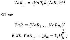
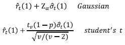
<body><![CDATA[<p>This  paper seeks, with information on daily returns of five assets of the Colombian  market from 01/03/2008 until 10/12/2010, to estimate a univariate and a  multivariate GARCH model for a portfolio, with information on daily returns of  five assets of the Colombian stock  market. Assigning equal weights for the asset returns, I use the VaR as a  portfolio risk measure, in order to make comparisons between the two models. </p>     <p>&nbsp;</p>     <p><font size="3"><b>I. Theoretical Framework</b></font></p>     <p><b>Value at Risk &#8211;VaR</b></p>     <p>The importance  of this measure lies in its usefulness for quantification of market risk and as  a regulatory tool, since the environment in which financial activity unfolds is  characterized by large fluctuations in prices of financial assets. In general,  the VaR is an indicator of the extreme points within which fluctuates the  profitability of an investment in an asset or a particular portfolio. That is,  represents the maximum loss incurred by an asset in the&alpha; * 100%  best cases (smaller losses). It is expected that the loss on the  investment does not exceed the VaR with probability &alpha;. </p>     <p> On the other  hand, VaR is a natural application of volatility models given that it depends  directly to the forecast of the conditional variance, consequently, the  estimation of the conditional distribution of returns becomes the main input  for the application of this methodology (Gall&oacute;n and G&oacute;mez, 2007). Using the  conditional mean and the conditional variance obtained from the estimated GARCH,  the quantiles of the conditional distribution can be easily obtained for the  calculation of VaR (Tsay, 2002).  According  to the distribution of errors, the VaR can be calculated as:</p>     <p align="center"><img src="/img/revistas/pece/n19/n19a4e0.jpg"></p>     <p>Where Z<sub>&alpha;</sub> is the <i>&alpha;<sup>th</sup></i> quantile of a standard normal distribution and <i>t<sub>v</sub>(1 - p)</i>, is the <i>(1 - p)<sup>th</sup></i> quantile of a <i>student's t</i> distribution with <i>v</i> degrees of freedom.</p>     <p> As mentioned by Tsay  (2002), VaR is associated with the prediction of a possible loss of a portfolio  for a given time horizon. Therefore, it should be calculated using the  distribution of forecasts of returns. Specifically, the VaR of the returns of a  portfolio, <i>r<sub>t</sub></i>, for a horizon <i>s</i> should be estimated based on forecasts of <i>r<sub>t+s</sub>(s)</i> given the information available at time <i>t</i>. The forecast of <i>r<sub>t+s</sub>(s)</i> depends on the model assumed to describe the  dynamics of returns, such as the ARCH model. </p>     <p> According with Alves,  Nogales and Ruiz (2009) the first decision one has to make when trying to  predict the VaR of a portfolio is whether to use a multivariate model for the  system of individual asset returns or, alternatively, to use a univariate  procedure for the portfolio returns. They argue that, as the dimension of the  portfolio increases, the usually large number of parameters involved renders  the estimation of multivariate models more complicated, compromising their  predictive ability.</p>     ]]></body>
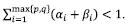
<body><![CDATA[<p><b>Univariate  GARCH models</b></p>     <p>First, it is  important to note some stylized facts of financial assets (in high frequency).  The distribution of returns is not normal: extreme returns occur most  frequently than expected under normality (fat tails) and extreme negative  returns occur most frequently than positive (negative asymmetry);  autocorrelations of the returns tend to be not significant, there are clusters  of volatility and calendar effects (Melo et al., 2005). According to (Tsay, 2010), a basic way to  represent this type of series would be:</p>     <p align="center"><img src="/img/revistas/pece/n19/n19a4e1.jpg"></p>     <p>Where &alpha;<sub>t</sub> is the <i>shock  or innovation </i>of the asset returns,  <i>r<sub>t</sub></i>, and &sigma;<sub>t</sub><sup>2</sup> is the process for the volatility of  <i>r<sub>t</sub></i>. Conditional heteroskedasticity  models center in the the dynamics of &sigma;<sub>t</sub><sup>2</sup>: The <i>volatility equation</i>. In order to do that, the specification in  equation (1) is the starting point. It can be expressed as:</p>     <p align="center"><img src="/img/revistas/pece/n19/n19a4e2.jpg"></p>     <p>Based on the  type of specification for equation (2), we can separate conditional  heteroskedastic models into (i) deterministic models ''that use an exact  function to govern the evolution of &sigma;<sub>t</sub><sup>2</sup>'' (Tsay, 2010, p. 100), or (ii)  stochastic models, that make &sigma;<sub>t</sub><sup>2</sup>  follow a random process. (G)ARCH and E-GARCH  models, for example, are located in the first group, while stochastic  volatility models, belong to the second group.</p>     <p>    <i>GARCH </i>(generalized autoregressive conditional  heteroskedastic) models have a  more flexible lags structure, and in many cases, allow a description more parsimonious  of the data than ARCH models.  In this  case, we keep the basic expression for innovations, and use the following  expression for the volatility equation: </p>     <p align="center"><img src="/img/revistas/pece/n19/n19a4e3.jpg"></p>     <p>&nbsp;</p>     <p>Where the  persistence of shocks to the volatility is given by the sum of &alpha;<sub>i</sub> and &beta;<sub>i</sub>. This expression is useful in  representing the clustering in volatility usually observed in series of  returns: a large shock in volatility yesterday increases the probability of a  large shock in today's volatility (Tsay, 2010). However, a drawback of this  model is that it does not allow for distinguishing between impacts of negative  and positive shocks, which tend to be different (leverage effect). Some  regularity conditions must be imposed to the model: &omega; &gt; 0, <i>&alpha;<sub>i</sub></i> <u>&gt;</u> 0, <i>&beta;<sub>f</sub></i> <u>&gt;</u> 0, <img src="/img/revistas/pece/n19/n19a4e3a.jpg">.</p>     ]]></body>

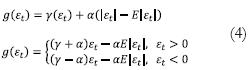
<body><![CDATA[<p> The positivity  restrictions are necessary for the conditional variance of the innovations to  exist, and for avoiding degeneration of their process &alpha;<sub>t</sub> (Carnero, Pe&ntilde;a, &amp; Ruiz, 2004). The last  constraint implies that the process is covariance stationary, and that its  marginal variance of innovations exists (&sigma;<sup>2</sup> &lt; &infin;), but its conditional variance, &sigma;<sub>t</sub><sup>2</sup>, evolves over time &#91; (Tsay, 2010)  (Carnero, Pe&ntilde;a, &amp; Ruiz, 2004)&#93;.</p>     <p> On the other  hand, the EGARCH model relaxes the positivity restrictions to its parameters  and allows for the treatment of leverage effects. In that sense, the EGARCH  considers the following specification for the weighted innovation:</p>     <p align="center"><img src="/img/revistas/pece/n19/n19a4e4.jpg"></p>     <p>Note that the  first term, related to  is a regular ARCH term and it determines the  sign of the effect, while the second one, linked to &alpha; is the asymmetric effect and it determines the  size of the effect. This specification succeeds at representing leverage  effects, since usually the estimated value of &gamma; is negative, which implies that |&gamma; - &alpha;|&gt;|&gamma; + &alpha;|. Now, in order to lose the  positivity constraints, the volatility equation is expressed in log terms. For  instance, in the case of EGARCH(1,1),  it  is given by:</p>     <p align="center"><img src="/img/revistas/pece/n19/n19a4e5.jpg"></p>     <p>Regarding  restrictions, the only restriction imposed on the parameters of the EGARCH is  that |&beta;| &lt; 1, so that the log-volatility  process is stationary.</p>     <p> Finally, as  mentioned above, given an estimated uniariate (G)ARCH model on a return  series, one knows the conditional distribution of returns, and one can forecast  the value-at-risk (VaR) of a long or short position. When considering a  portfolio of assets, the portfolio return can be computed directly from the  asset shares and returns (Bauwens et al., 2006). </p>     <p><b>Multivariate  GARCH models</b></p>     <p>A multivariate <i>GARCH(p,q) </i>model, <i>MGARCH(p,q)</i>, can be represented as: </p>     <p align="center"><img src="/img/revistas/pece/n19/n19a4e6.jpg"></p>     ]]></body>
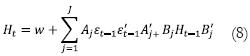
<body><![CDATA[<p>Where <i>H<sub>t</sub></i><sup>1/2</sup> is the conditional covariance matrix of <i>Y<sub>t</sub></i> (series of returns) and &epsilon;<sub>t</sub> is a vector of white noise processes such that E(&epsilon;<sub>t</sub>) = 0 and E(<i>&epsilon;<sub>t</sub>&epsilon;</i>'<sub>t</sub>) = 1. There are two kinds of  multivariate GARCH models: one type models the time-varying covariances and the  second type models the conditional correlations (Tsay, 2010).</p>     <p> The most direct  generalization of the univariate GARCH(1,1) model is the VEC model given by:</p>     <p align="center"><img src="/img/revistas/pece/n19/n19a4e7.jpg"></p>     <p>where the vec  operator allows each cross-product to influence each covariance term. The VEC  model is covariance stationary if the modulus of the eigenvalues of A+B are  less than one.</p>     <p> One of the main drawbacks  of the multivariate models, and from this in particular, is that the number of  parameters to be estimated is too large. Therefore, the DVEC model restricts  the matrices A and B to be diagonal. In this case, each element <i>h<sub>ijt</sub></i> depends only on its own lag and on the  previous value <i>&epsilon;<sub>it</sub>&epsilon;<sub>jt</sub></i>. However, this model is not  suitable to represent volatility transmissions between assets and in both VEC  and DVEC models it is difficult to guarantee the positiveness of  <i>H<sub>t</sub></i> (Tsay, 2010).</p>     <p> Another usual  specification is the BEKK model based on quadratic forms:</p>     <p align="center"><img src="/img/revistas/pece/n19/n19a4e8.jpg"></p>     <p>The full BEKK becomes  intractable as the number of assets grows. However, the diagonal BEKK partially  addresses some of the number of parameters by restricting A and B to be  diagonal.</p>     <p> Finally, the  last multivariate model that is going to be considered here is the Constant  Conditional Correlation (CCC), which uses a different approach: it decomposes  the conditional covariance into the conditional variances and the conditional  correlation, which is assumed to be constant:</p>     <p align="center"><img src="/img/revistas/pece/n19/n19a4e9.jpg"></p>     ]]></body>
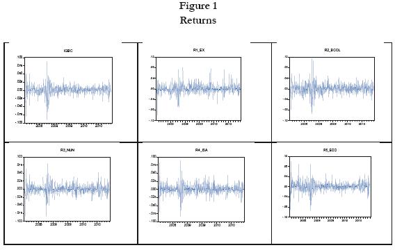
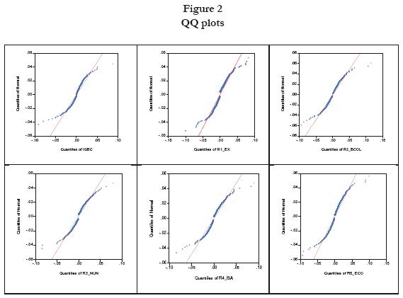
<body><![CDATA[<p>Where is a diagonal matrix with the conditional  standard deviation of the <i>i<sup>th</sup></i> asset on its diagonal position. In this model, the conditional variances are  typically model using standard GARCH(1,1) models:</p>     <p align="center"><img src="/img/revistas/pece/n19/n19a4e10.jpg"></p>     <p>&nbsp;</p>     <p><font size="3"><b>II. Estimation and Results</b></font></p>     <p><b>Data</b></p>     <p>In this paper I  consider some of the five most tradable assets in the stock exchange in  Colombia. The returns of these assets were calculated from the logarithmic  difference of the price. These returns are for &Eacute;xito, Bancolombia,  Nutresa, Isa and Ecopetrol. Additionally  I consider the IGBC<a href="#_ftn1" name="_ftnref1"><sup>1</sup></a> &#8211;&Iacute;ndice General de la Bolsa de Valores de Colombia&#8211;, to compare it with the  results obtained by forming a portfolio with equal weights for those returns. The  data has daily frequency from 03/01/2008 until 10/12/2012 for a total of 758  data. Below are the plots of the returns and the descriptive statistics.</p>     <p>In all cases I  apply stationarity tests (Dickey-Fuller and Phillips-Perron) and reject the  unit root null hypothesis. Below are the QQ plots of returns. It compares the  observed quantiles with the theoretical quantiles of a normal distribution. Therefore,  if the distribution of the series is normal it should be a straight line. </p>     <p align="center"><a name="f1"></a><img src="/img/revistas/pece/n19/n19a4f1.jpg"></p>     <p align="center"><a name="f2"></a><img src="/img/revistas/pece/n19/n19a4f2.jpg"></p>     <p>&nbsp;</p>     ]]></body>
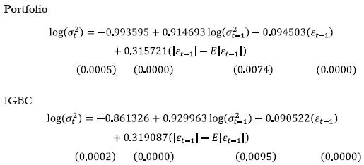
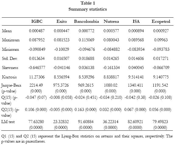
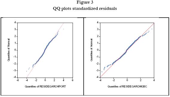
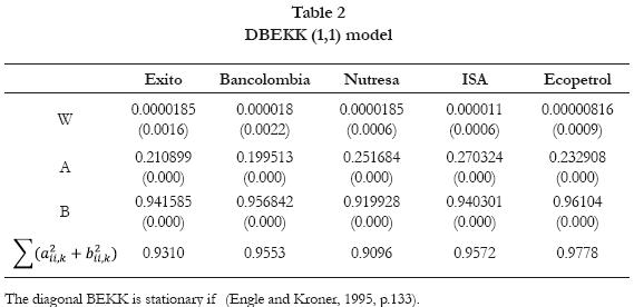
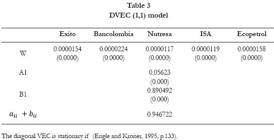
<body><![CDATA[<p>In this <a href="#f1">Figure</a>,  there is a pattern of ''S rotated'' in all cases, where the greatest differences  with respect to dotted line are at the extremes. This result indicates that the  distributions of the series have tails heavier than those of a normal distribution.  Below there is a summary of statistics for each return:</p>     <p align="center"><a name="t1"></a><img src="/img/revistas/pece/n19/n19a4t1.jpg"></p>     <p>&nbsp;</p>     <p>Considering the  standard deviation as a measure of volatility, more volatile returns correspond  to, in order, Bancolombia, Ecopetrol and Exito.  On the other hand, according to the  coefficients of skewness and kurtosis, the Jarque-Bera statistic and QQ plots,  one cannot assume normality of returns. Additionally, according to the  Ljung-Box statistics we cannot reject the null hypothesis of no autocorrelation  up to order 15 in the series of returns but is rejected in the squared returns.  Finally, to confirm whether there are ARCH effects, was applied the Lagrange  multiplier test (LM test), which considers the null hypothesis of no ARCH  errors versus the alternative hypothesis that the conditional error variance is  given by an ARCH process. The null hypothesis is rejected in all cases,  confirming ARCH effects in the errors.</p>     <p> In the  estimation, first, I consider two univariate models, one for the IGBC and one  for the portfolio assuming equal weights for assets. In both cases I tested  various specifications and the model with best fit given the constraints of the  parameters, the significance of the conditional volatility and the AIC and SC  criteria was an EGARCH (1,1) with student's errors.</p>     <p align="center"><img src="/img/revistas/pece/n19/n19a4e11.jpg"></p>     <p>The fact that  both series have similar behavior has sense because the portfolio was  constructed from some of the more tradable assets in the Colombian market and  IGBC is an indicator that measures just that. In both cases it holds that &Beta; &lt; 1  (significant) and is verified that there are  leverage effects due to the parameter &gamma; is negative, so the effect on volatility is bigger when the return  is negative than when it is positive. Below are the QQ plots of the  standardized residuals. It is observed that normality for the standardized  residuals is still being rejected due to the excess of kurtosis but in a lower  degree.</p>     <p>In order to  check the specification in the conditional variance function in both models I  used the LM test, finding evidence for the absence of additional ARCH effects, confirming  that the EGARCH (1,1)<a href="#_ftn2" name="_ftnref2"><sup>2</sup></a> fits well.</p>     <p> In the  multivariate case, three specifications were chosen to model the distribution  of conditional covariance matrix of the returns of the five assets, : DVEC,  DBEKK and CCC models. The choice of these  models is not only because in relative terms they are simpler to estimate, but  also because the cross-correlation of returns<a href="#_ftn3" name="_ftnref3"><sup>3</sup></a> does not confirm a significant linear relation both contemporary and in the  first lag, so there seems not to exist an important cross-influence on the  markets. Additionally, I used the LM test and I found evidence for the  existence of multivariate ARCH effects (at 5% significance). Then, I proceed to  estimate the MGARCH models and the results are presented bellow. In all cases,  the stationarity conditions are verified.</p>      <p align="center"><a name="f3"></a><img src="/img/revistas/pece/n19/n19a4f3.jpg"></p>     ]]></body>
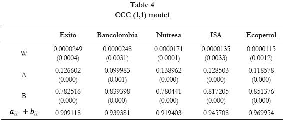
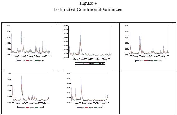
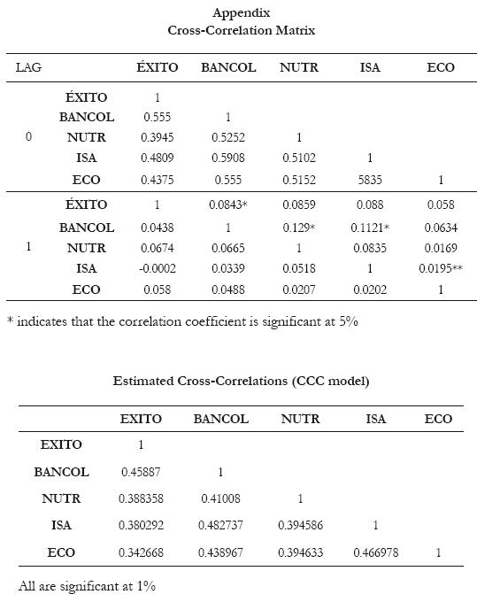
<body><![CDATA[<p>&nbsp;</p>     <p align="center"><a name="t2"></a><img src="/img/revistas/pece/n19/n19a4t2.jpg"></p>     <p align="center">&nbsp;</p>     <p align="center"><a name="t3"></a><img src="/img/revistas/pece/n19/n19a4t3.jpg"></p>     <p align="center">&nbsp;</p>     <p align="center"><a name="t4"></a><img src="/img/revistas/pece/n19/n19a4t4.jpg"></p>     <p>&nbsp;</p>     <p>The stationarity  conditions are the same as in the univariate GARCH model <i>W &gt; 0, &alpha;, &beta; <u>&gt;</u> 0, a<sub>ii</sub> + b<sub>ii</sub> &lt; </i>1. In the <a href="#a1">Appendix</a> are the results  for the estimated cross-correlation matrix from the CCC model.</p>     <p> The plots of the  estimated conditional variances from the three models are presented below.</p>     <p align="center"><a name="f4"></a><img src="/img/revistas/pece/n19/n19a4f4.jpg"></p>     ]]></body>
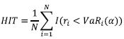
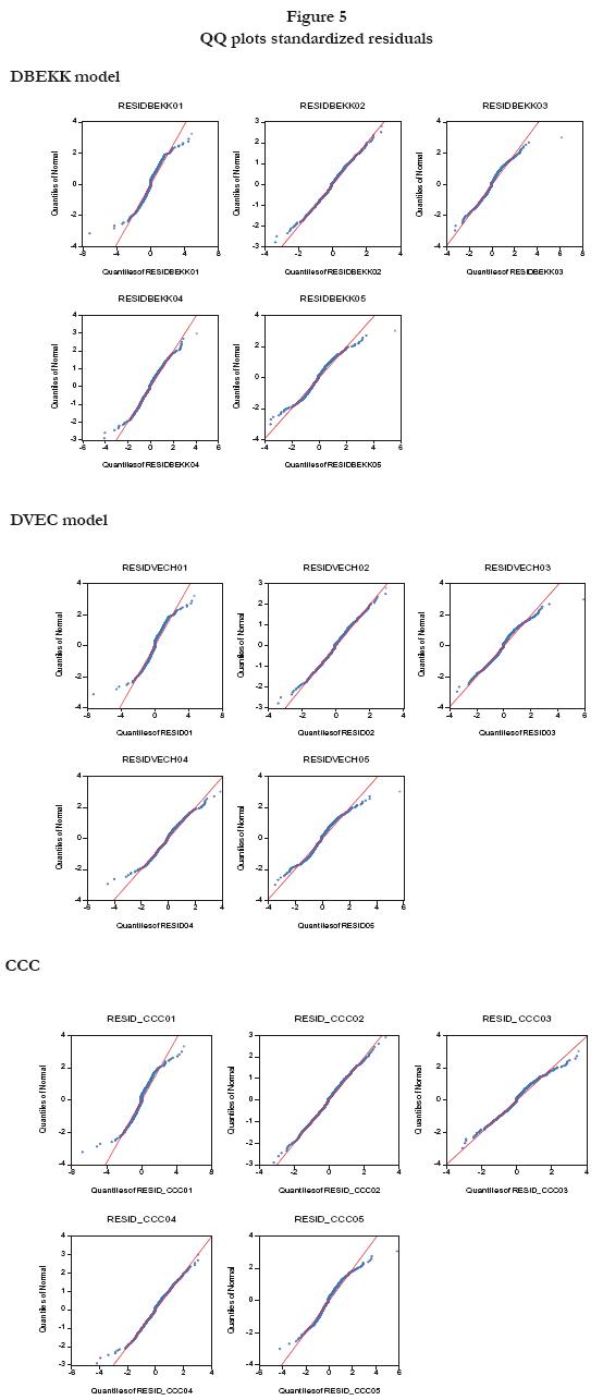
<body><![CDATA[<p align="center">&nbsp;</p>     <p>In conclusion,  it seems clear that the estimated conditional covariance matrices of the models  are very close, however there is uncertainty about which of the models is  better. In addition, QQ plots of standardized residuals are presented below,  which are showing excess kurtosis in some cases with a result similar to the  univariate models.</p>     <p>Once established  the processes that model the dependence of returns, it is possible to calculate  risk measures and then verify their performance through backtesting. Given the  results presented above the VaR was estimated assuming that the distribution of  the errors is a Student's , according to the methodology  previously presented. In the multivariate case, following Gall&oacute;n and G&oacute;mez  (2007), the VaR for a portfolio consisting of N assets in a time horizon with probability is defined as:</p>     <p align="center"><img src="/img/revistas/pece/n19/n19a4e12.jpg"></p>     <p>&nbsp;</p>     <p align="center"><a name="f5"></a><img src="/img/revistas/pece/n19/n19a4f5.jpg"></p>     <p>&nbsp;</p>     <p>  Where <i>w<sub>i</sub></i> is the amount invested in the <i>i<sup>th</sup></i> asset. Here it is assumed that is <i>w<sub>i</sub></i> equal for all assets, in order to compare it  with the portfolio estimated in the univariate case and the IGBC. </p>     <p> A basic measure  for comparing the estimated models is the failure ratio or HIT, defined as</p>     <p align="center"><img src="/img/revistas/pece/n19/n19a4e13.jpg"></p>     ]]></body>
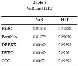
<body><![CDATA[<p>Where <i>l</i>(<i>r<sub>i</sub></i> &lt; VaR<sub>i</sub>(&alpha;))is an indicator variable that takes the value  1 when <i>r<sub>i</sub></i> &lt; VaR<sub>i</sub>(&alpha;). A model is correctly specified  when this ratio is equal to the pre-specified probability for the VaR. Below is the result of the estimate for a confidence  level of 95%.</p>     <p align="center"><a name="t5"></a><img src="/img/revistas/pece/n19/n19a4t5.jpg"></p>     <p>&nbsp;</p>     <p>For instance the  VaR of the portfolio indicates that the maximum loss expected with a  probability of 95% and a horizon of one day shall not exceed that percentage of  the amount invested. The HIT calculated shows that the models that are closer  to 95% pre-specified for the VaR are both models that were obtained from the  univariate (E)GARCH. Additionally it is noted that similar results are obtained  for the three multivariate specifications. Finally, the most important result  is that the univariate models perform better in estimating the VaR than the  multivariate models, which seems to underestimate the risk of the portfolio.</p>     <p>&nbsp;</p>     <p><font size="3"><b>Conclusions</b></font></p>     <p>The modeling of  risk and volatility of financial instruments has become a major area of  research in last decades. This study sought to estimate the risk of a  portfolio consisting of 5 assets of the Colombian stock market. In the  estimation, I considered two univariate models, one for the IGBC and one for  the portfolio assuming equal weights for assets. In the multivariate case,  three specifications were chosen to model the distribution of conditional  covariance matrix of the returns of the five assets: DVEC, DBEKK and CCC  models. Once established the processes that model the dependence of returns, the  VaR was estimated.</p>     <p> Results show how  univariate models performed better in estimating the VaR than the multivariate  models, which seems to underestimate the risk of the portfolio. However, the  results are subject to the number of assets and the estimated multivariate  models. In that sense, it would be interesting to consider more assets to make the  estimation and use other multivariate GARCH specifications. Additionally, one could  apply more sophisticated backtesting techniques and out of sample analysis. Finally,  for comparisons would be interesting to consider more elaborated measures for  the calculation of VaR such as the Conditional Autoregressive VaR (CaViaR).</p>     <p>&nbsp;</p> <hr noshade size="1">     <p><font size="3"> <b>NOTAS</b></font></p>     ]]></body>
<body><![CDATA[<p><a href="#_ftnref0" name="_ftn0">*</a> El art&iacute;culo no tiene una investigaci&oacute;n previa.</p>     <p> <a href="#_ftnref1" name="_ftn1" >1</a> This  is the result of weighting the more liquid shares with higher capitalization  traded on the stock market.</p>       <p>    <a href="#_ftnref2" name="_ftn2" >2</a> For the IGBC the contrast  yields a value of 1.759175 (0.1847) and for the portfolio 0.512384 (0.4741). </p>         <p><a href="#_ftnref3" name="_ftn3" >3</a> See <a href="#a1">Appendix</a></p> <hr noshade size="1">     <p>&nbsp;</p>     <p><font size="3"><b>References</b></font></p>     <!-- ref --><p>Alves, A.; Nogales, F.; Ruiz, E. (2009). ''Comparing  univariate and multivariate models to forecast portfolio value-at-risk''.  Statistics  and Econometrics Working Papers ws097222, Universidad Carlos III, Departamento  de Estad&iacute;stica y Econometr&iacute;a.    &nbsp;&nbsp;&nbsp;&nbsp;&nbsp;&nbsp;&nbsp;&nbsp;[&#160;<a href="javascript:void(0);" onclick="javascript: window.open('/scielo.php?script=sci_nlinks&ref=000129&pid=S1657-4214201200010000400001&lng=','','width=640,height=500,resizable=yes,scrollbars=1,menubar=yes,');">Links</a>&#160;]<!-- end-ref --></p>     <!-- ref --><p> Bauwens, L.; Laurent, S.;  Rombouts, J. (2006). ''Multivariate GARCH models: A  survey''.  <i>Journal of Applied Econometrics</i>, 21, 79-109p.    &nbsp;&nbsp;&nbsp;&nbsp;&nbsp;&nbsp;&nbsp;&nbsp;[&#160;<a href="javascript:void(0);" onclick="javascript: window.open('/scielo.php?script=sci_nlinks&ref=000131&pid=S1657-4214201200010000400002&lng=','','width=640,height=500,resizable=yes,scrollbars=1,menubar=yes,');">Links</a>&#160;]<!-- end-ref --></p>     ]]></body>
<body><![CDATA[<!-- ref --><p> Bera, A. K.; Kim, S.  (2002). ''Testing constancy of correlation and other specifications of the  BGARCH model with an application to international equity returns''. <i>Journal of Empirical Finance</i> 9, 171&#8211;175.    &nbsp;&nbsp;&nbsp;&nbsp;&nbsp;&nbsp;&nbsp;&nbsp;[&#160;<a href="javascript:void(0);" onclick="javascript: window.open('/scielo.php?script=sci_nlinks&ref=000133&pid=S1657-4214201200010000400003&lng=','','width=640,height=500,resizable=yes,scrollbars=1,menubar=yes,');">Links</a>&#160;]<!-- end-ref --></p>     <!-- ref --><p> Bollerslev, T.; Engle, R.;  Nelson, D. (1994). ''ARCH models''. En MacFadden, D.  F., Engle, R. E. (Eds.), <i>Handbook of  Econometrics</i>, Vol. 4. North-Holland: Amsterdam.    &nbsp;&nbsp;&nbsp;&nbsp;&nbsp;&nbsp;&nbsp;&nbsp;[&#160;<a href="javascript:void(0);" onclick="javascript: window.open('/scielo.php?script=sci_nlinks&ref=000135&pid=S1657-4214201200010000400004&lng=','','width=640,height=500,resizable=yes,scrollbars=1,menubar=yes,');">Links</a>&#160;]<!-- end-ref --></p>     <!-- ref --><p> Carnero,  M. A.; Pe&ntilde;a, D.; Ruiz, E.  (2004). ''Persistence and Kurtosis in GARCH and  Stochastic Volatility Models''. <i>Journal of  Financial Econometrics</i>, 2 (2), 319-342.    &nbsp;&nbsp;&nbsp;&nbsp;&nbsp;&nbsp;&nbsp;&nbsp;[&#160;<a href="javascript:void(0);" onclick="javascript: window.open('/scielo.php?script=sci_nlinks&ref=000137&pid=S1657-4214201200010000400005&lng=','','width=640,height=500,resizable=yes,scrollbars=1,menubar=yes,');">Links</a>&#160;]<!-- end-ref --></p>     <!-- ref --><p> Engle, E.  (1982). ''Autoregressive conditional heteroskedasticity with estimates of the  variance of United Kingdom inflation<i>''.  Econometrica</i> 50, 987&#8211;1008.    &nbsp;&nbsp;&nbsp;&nbsp;&nbsp;&nbsp;&nbsp;&nbsp;[&#160;<a href="javascript:void(0);" onclick="javascript: window.open('/scielo.php?script=sci_nlinks&ref=000139&pid=S1657-4214201200010000400006&lng=','','width=640,height=500,resizable=yes,scrollbars=1,menubar=yes,');">Links</a>&#160;]<!-- end-ref --></p>     <!-- ref --><p> Engle, R.; Kroner, K.  (1995). ''Multivariate Simultaneous Generalized ARCH''. <i>Econometric Theory </i>Vol. 11, No. 1, pp. 122-150.    &nbsp;&nbsp;&nbsp;&nbsp;&nbsp;&nbsp;&nbsp;&nbsp;[&#160;<a href="javascript:void(0);" onclick="javascript: window.open('/scielo.php?script=sci_nlinks&ref=000141&pid=S1657-4214201200010000400007&lng=','','width=640,height=500,resizable=yes,scrollbars=1,menubar=yes,');">Links</a>&#160;]<!-- end-ref --></p>     ]]></body>
<body><![CDATA[<!-- ref --><p> Engle, R.; Patton, A.  (2001). ''What good is a volatility model?'' <i>Quantitative Finance</i> 1, 237&#8211;245.    &nbsp;&nbsp;&nbsp;&nbsp;&nbsp;&nbsp;&nbsp;&nbsp;[&#160;<a href="javascript:void(0);" onclick="javascript: window.open('/scielo.php?script=sci_nlinks&ref=000143&pid=S1657-4214201200010000400008&lng=','','width=640,height=500,resizable=yes,scrollbars=1,menubar=yes,');">Links</a>&#160;]<!-- end-ref --></p>     <!-- ref --><p> Gall&oacute;n, S.; G&oacute;mez, K. (2007). ''Distribuci&oacute;n condicional de los retornos de la  tasa de cambio colombiana: un ejercicio emp&iacute;rico a partir de modelos GARCH  multivariados''. <i>Revista de Econom&iacute;a del  Rosario,</i> Vol. 10, No. 2.    &nbsp;&nbsp;&nbsp;&nbsp;&nbsp;&nbsp;&nbsp;&nbsp;[&#160;<a href="javascript:void(0);" onclick="javascript: window.open('/scielo.php?script=sci_nlinks&ref=000145&pid=S1657-4214201200010000400009&lng=','','width=640,height=500,resizable=yes,scrollbars=1,menubar=yes,');">Links</a>&#160;]<!-- end-ref --></p>     <!-- ref --><p> Ghysels, E.; Harvey, A.;  Renault, E. (1996). ''Stochastic Volatility''. En  Maddala, G. S., Rao, C. R., Vinod, H. D., (Eds.), <i>Handbook of Statistics</i>, Vol. 14: statistical methods in finance. North-Holland: Amsterdam: 119&#8211;91.    &nbsp;&nbsp;&nbsp;&nbsp;&nbsp;&nbsp;&nbsp;&nbsp;[&#160;<a href="javascript:void(0);" onclick="javascript: window.open('/scielo.php?script=sci_nlinks&ref=000147&pid=S1657-4214201200010000400010&lng=','','width=640,height=500,resizable=yes,scrollbars=1,menubar=yes,');">Links</a>&#160;]<!-- end-ref --></p>     <!-- ref --><p> Melo, L.; Becerra, O. (2005). ''Medidas de riesgo, caracter&iacute;sticas y  t&eacute;cnicas de medici&oacute;n: una aplicaci&oacute;n del VaR y el ES a la tasa interbancaria de  Colombia''. <i>Borradores de Econom&iacute;a</i> 343, Banco de la Republica de Colombia, 75 p.    &nbsp;&nbsp;&nbsp;&nbsp;&nbsp;&nbsp;&nbsp;&nbsp;[&#160;<a href="javascript:void(0);" onclick="javascript: window.open('/scielo.php?script=sci_nlinks&ref=000149&pid=S1657-4214201200010000400011&lng=','','width=640,height=500,resizable=yes,scrollbars=1,menubar=yes,');">Links</a>&#160;]<!-- end-ref --></p>     <!-- ref --><p> Tsay, R.  (2002). ''<i>Analysis of Financial Time Series</i>.'' John Wiley &amp; Sons.    &nbsp;&nbsp;&nbsp;&nbsp;&nbsp;&nbsp;&nbsp;&nbsp;[&#160;<a href="javascript:void(0);" onclick="javascript: window.open('/scielo.php?script=sci_nlinks&ref=000151&pid=S1657-4214201200010000400012&lng=','','width=640,height=500,resizable=yes,scrollbars=1,menubar=yes,');">Links</a>&#160;]<!-- end-ref --></p>     ]]></body>
<body><![CDATA[<!-- ref --><p> Tsay, R.  (2010). Analysis of Financial Time Series. Chicago: John Wiley &amp; Sons, Inc.    &nbsp;&nbsp;&nbsp;&nbsp;&nbsp;&nbsp;&nbsp;&nbsp;[&#160;<a href="javascript:void(0);" onclick="javascript: window.open('/scielo.php?script=sci_nlinks&ref=000153&pid=S1657-4214201200010000400013&lng=','','width=640,height=500,resizable=yes,scrollbars=1,menubar=yes,');">Links</a>&#160;]<!-- end-ref --></p>     <p>&nbsp;</p>     <p>&nbsp;</p>     <p><font size="3"> <b>Appendix</b></font></p>     <p align="center"><a name="a1"></a><img src="/img/revistas/pece/n19/n19a4a1.jpg"></p>     <p>&nbsp;</p> </font>      ]]></body><back>
<ref-list>
<ref id="B1">
<nlm-citation citation-type="">
<person-group person-group-type="author">
<name>
<surname><![CDATA[Alves]]></surname>
<given-names><![CDATA[A.]]></given-names>
</name>
<name>
<surname><![CDATA[Nogales]]></surname>
<given-names><![CDATA[F.]]></given-names>
</name>
<name>
<surname><![CDATA[Ruiz]]></surname>
<given-names><![CDATA[E.]]></given-names>
</name>
</person-group>
<source><![CDATA[''Comparing univariate and multivariate models to forecast portfolio value-at-risk'']]></source>
<year>2009</year>
</nlm-citation>
</ref>
<ref id="B2">
<nlm-citation citation-type="journal">
<person-group person-group-type="author">
<name>
<surname><![CDATA[Bauwens]]></surname>
<given-names><![CDATA[L.]]></given-names>
</name>
<name>
<surname><![CDATA[Laurent]]></surname>
<given-names><![CDATA[S.]]></given-names>
</name>
<name>
<surname><![CDATA[Rombouts]]></surname>
<given-names><![CDATA[J.]]></given-names>
</name>
</person-group>
<article-title xml:lang="en"><![CDATA[Multivariate GARCH models: A survey]]></article-title>
<source><![CDATA[Journal of Applied Econometrics]]></source>
<year>2006</year>
<volume>21</volume>
<page-range>79-109</page-range></nlm-citation>
</ref>
<ref id="B3">
<nlm-citation citation-type="journal">
<person-group person-group-type="author">
<name>
<surname><![CDATA[Bera]]></surname>
<given-names><![CDATA[A. K.]]></given-names>
</name>
<name>
<surname><![CDATA[Kim]]></surname>
<given-names><![CDATA[S.]]></given-names>
</name>
</person-group>
<article-title xml:lang="en"><![CDATA[''Testing constancy of correlation and other specifications of the BGARCH model with an application to international equity returns'']]></article-title>
<source><![CDATA[Journal of Empirical Finance]]></source>
<year>2002</year>
<volume>9</volume>
<page-range>171-175</page-range></nlm-citation>
</ref>
<ref id="B4">
<nlm-citation citation-type="">
<person-group person-group-type="author">
<name>
<surname><![CDATA[Bollerslev]]></surname>
<given-names><![CDATA[T.]]></given-names>
</name>
<name>
<surname><![CDATA[Engle]]></surname>
<given-names><![CDATA[R.]]></given-names>
</name>
<name>
<surname><![CDATA[Nelson]]></surname>
<given-names><![CDATA[D.]]></given-names>
</name>
</person-group>
<article-title xml:lang="en"><![CDATA[''ARCH models'']]></article-title>
<person-group person-group-type="editor">
<name>
<surname><![CDATA[MacFadden]]></surname>
<given-names><![CDATA[D. F.]]></given-names>
</name>
<name>
<surname><![CDATA[Engle]]></surname>
<given-names><![CDATA[R. E.]]></given-names>
</name>
</person-group>
<source><![CDATA[Handbook of Econometrics]]></source>
<year>1994</year>
<volume>4</volume>
<publisher-loc><![CDATA[North-Holland^eAmsterdam Amsterdam]]></publisher-loc>
</nlm-citation>
</ref>
<ref id="B5">
<nlm-citation citation-type="journal">
<person-group person-group-type="author">
<name>
<surname><![CDATA[Carnero]]></surname>
<given-names><![CDATA[M. A.]]></given-names>
</name>
<name>
<surname><![CDATA[Peña]]></surname>
<given-names><![CDATA[D.]]></given-names>
</name>
<name>
<surname><![CDATA[Ruiz]]></surname>
<given-names><![CDATA[E.]]></given-names>
</name>
</person-group>
<article-title xml:lang="en"><![CDATA[''Persistence and Kurtosis in GARCH and Stochastic Volatility Models'']]></article-title>
<source><![CDATA[Journal of Financial Econometrics]]></source>
<year>2004</year>
<volume>2</volume>
<numero>2</numero>
<issue>2</issue>
<page-range>319-342</page-range></nlm-citation>
</ref>
<ref id="B6">
<nlm-citation citation-type="journal">
<person-group person-group-type="author">
<name>
<surname><![CDATA[Engle]]></surname>
<given-names><![CDATA[E.]]></given-names>
</name>
</person-group>
<article-title xml:lang="en"><![CDATA[''Autoregressive conditional heteroskedasticity with estimates of the variance of United Kingdom inflation'']]></article-title>
<source><![CDATA[Econometrica]]></source>
<year>1982</year>
<volume>50</volume>
<page-range>987-1008</page-range></nlm-citation>
</ref>
<ref id="B7">
<nlm-citation citation-type="journal">
<person-group person-group-type="author">
<name>
<surname><![CDATA[Engle]]></surname>
<given-names><![CDATA[R.]]></given-names>
</name>
<name>
<surname><![CDATA[Kroner]]></surname>
<given-names><![CDATA[K.]]></given-names>
</name>
</person-group>
<article-title xml:lang="en"><![CDATA[''Multivariate Simultaneous Generalized ARCH'']]></article-title>
<source><![CDATA[Econometric Theory]]></source>
<year>1995</year>
<volume>11</volume>
<numero>1</numero>
<issue>1</issue>
<page-range>122-150</page-range></nlm-citation>
</ref>
<ref id="B8">
<nlm-citation citation-type="journal">
<person-group person-group-type="author">
<name>
<surname><![CDATA[Engle]]></surname>
<given-names><![CDATA[R.]]></given-names>
</name>
<name>
<surname><![CDATA[Patton]]></surname>
<given-names><![CDATA[A.]]></given-names>
</name>
</person-group>
<article-title xml:lang="en"><![CDATA[''What good is a volatility model?'']]></article-title>
<source><![CDATA[Quantitative Finance]]></source>
<year>2001</year>
<volume>1</volume>
<page-range>237-245</page-range></nlm-citation>
</ref>
<ref id="B9">
<nlm-citation citation-type="journal">
<person-group person-group-type="author">
<name>
<surname><![CDATA[Gallón]]></surname>
<given-names><![CDATA[S.]]></given-names>
</name>
<name>
<surname><![CDATA[Gómez]]></surname>
<given-names><![CDATA[K.]]></given-names>
</name>
</person-group>
<article-title xml:lang="es"><![CDATA[''Distribución condicional de los retornos de la tasa de cambio colombiana: un ejercicio empírico a partir de modelos GARCH multivariados'']]></article-title>
<source><![CDATA[Revista de Economía del Rosario]]></source>
<year>2007</year>
<volume>10</volume>
<numero>2</numero>
<issue>2</issue>
</nlm-citation>
</ref>
<ref id="B10">
<nlm-citation citation-type="">
<person-group person-group-type="author">
<name>
<surname><![CDATA[Ghysels]]></surname>
<given-names><![CDATA[E.]]></given-names>
</name>
<name>
<surname><![CDATA[Harvey]]></surname>
<given-names><![CDATA[A.]]></given-names>
</name>
<name>
<surname><![CDATA[Renault]]></surname>
<given-names><![CDATA[E.]]></given-names>
</name>
</person-group>
<article-title xml:lang="en"><![CDATA[''Stochastic Volatility'']]></article-title>
<person-group person-group-type="editor">
<name>
<surname><![CDATA[Maddala]]></surname>
<given-names><![CDATA[G. S.]]></given-names>
</name>
<name>
<surname><![CDATA[Rao]]></surname>
<given-names><![CDATA[C. R.]]></given-names>
</name>
<name>
<surname><![CDATA[Vinod]]></surname>
<given-names><![CDATA[H. D.]]></given-names>
</name>
</person-group>
<source><![CDATA[Handbook of Statistics]]></source>
<year>1996</year>
<volume>14</volume>
<page-range>119-91</page-range><publisher-loc><![CDATA[Amsterdam ]]></publisher-loc>
</nlm-citation>
</ref>
<ref id="B11">
<nlm-citation citation-type="journal">
<person-group person-group-type="author">
<name>
<surname><![CDATA[Melo]]></surname>
<given-names><![CDATA[L.]]></given-names>
</name>
<name>
<surname><![CDATA[Becerra]]></surname>
<given-names><![CDATA[O.]]></given-names>
</name>
</person-group>
<article-title xml:lang="es"><![CDATA[''Medidas de riesgo, características y técnicas de medición: una aplicación del VaR y el ES a la tasa interbancaria de Colombia'']]></article-title>
<source><![CDATA[Borradores de Economía]]></source>
<year>2005</year>
<volume>343</volume>
<page-range>75</page-range><publisher-name><![CDATA[Banco de la Republica de Colombia]]></publisher-name>
</nlm-citation>
</ref>
<ref id="B12">
<nlm-citation citation-type="book">
<person-group person-group-type="author">
<name>
<surname><![CDATA[Tsay]]></surname>
<given-names><![CDATA[R.]]></given-names>
</name>
</person-group>
<source><![CDATA[''Analysis of Financial Time Series.'']]></source>
<year>2002</year>
<publisher-name><![CDATA[John Wiley & Sons]]></publisher-name>
</nlm-citation>
</ref>
<ref id="B13">
<nlm-citation citation-type="book">
<person-group person-group-type="author">
<name>
<surname><![CDATA[Tsay]]></surname>
<given-names><![CDATA[R.]]></given-names>
</name>
</person-group>
<source><![CDATA[Analysis of Financial Time Series]]></source>
<year>2010</year>
<publisher-loc><![CDATA[Chicago ]]></publisher-loc>
<publisher-name><![CDATA[John Wiley & Sons, Inc]]></publisher-name>
</nlm-citation>
</ref>
</ref-list>
</back>
</article>