


 English (pdf)
 Article in xml format
 Article references
 Send this article by e-mail
 Cited by SciELO
  Cited by Google
  Similars in
SciELO
Similars in
SciELO  Similars in Google
 Permalink
1. Introduction
Total losses are made up of two components; a component called Technical Losses (TechL) and another called Non-Technical Losses (NTechL). The legislative reform applied to the electricity industry in all its voltage levels, allowed the creation of different segments considered as business units, each one with its market characteristics and therefore with its own fundamentals in determining costs. In the field of the distribution segment, the Argentine regulatory standards introduced the concept of service quality based on a series of reliability indices, where the most important and descriptive parameter is the continuity of the electricity supply, leaving aside the considerations necessary to treatment the total losses. Of both components, the real difficulty arises in the determination of Non-Technical Losses (NTechL), due to the multiple factors that intervene within a general context that includes the economic, social and regulatory conditions where the company develops its activities, in addition to an abstract methodology that does not address the requirement of a technical analysis; administrative and commercial. In the state of the art there are not many specific studies on these losses, currently approached with a linear approximation methodology, where the final result of this is included as a significant percentage of total losses and leaving aside numerous directly incident variables such as: economic situation of the population; economic-financial situation of the company; energy purchase price; regulatory regime; etc. This new theoretical aspect for the treatment of this issue applicable to the regulation, is supported by the few considerations to quantify this type of losses that generate a cost component that is not measured due to the absence of an analytical profile that affects the correct analysis. of the economic-financial situation of the electricity companies. Therefore, the following points are presented that describe in a simplified way the problem and the new proposal for the treatment of variables:
The electricity market currently considers phenomena as linear, negatively influencing the parameters taken as a reference to set the quality of service.
Technological progress requires a transformation in the sector, especially at the level of regulatory entities, where to adopt stochastic approaches due to the existence of variables that present a certain dispersion is a necessity.
The use of a neural network to perform the calculation and determination of the error matrix during its training using the first derivation of the Widrow-Hoff rule of stochastic approximation would constitute a reference in the required transformation.
This work proposes a structure organized into sections, where in the sections 2nd and 3th describe the structure of the distribution segment and the theoretical aspect of the tools currently used, in the 4th and 5th a stratification for the identification of the origin of non-technical losses is developed and the theoretical presentation of the neural network. Finally, in the 6nd and 7 the details of the calculations and the most relevant conclusions are presented respectively.
2. Structure of the distribution segment. Natural monopolies
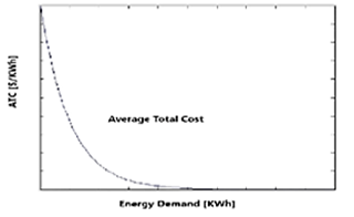
The problem of the current context in the distribution segment is characterized by the regulation mechanism and the restrictions imposed by a regulatory entity, which defines the general guidelines based on different legal limitations applied to business units that operate under the name of natural monopolies. The obligation of these to comply with a certain quality of service in the supply, lead to omitting certain aspects that in the first instance should be dealt with technically and then adapt them to the regulatory context. A natural monopoly arises when a company can offer a good or provide a service at a lower cost than two or more in the same sector and there is also an economy of scale in the production interval. The cost taken as a parameter to create a natural monopoly [4] is the average total cost.
A simple description of the situation, if two or more electricity distribution companies compete to provide service to a specific region, each one must build its own distribution network, generating higher total costs in the segment. Assuming that a single company is in charge of the construction of the electrical network, during its expansion process it must build more kilometers of lines for an increasing demand (Q), so the total cost is divided by an amount each time most users. In the same way as competitive companies [4], the relation between the total cost (fixed and variable) with respect to the demand, defines the average total cost, which one decreases as the number of users increases. The concept of average total cost is also applicable to natural monopolies, but with respect to competitive companies, its curve does not have the characteristic U aspect but rather the aspect shown in Fig. 1.
Another concept considered is the demand and the response of both types of companies to it. Characteristic of competitive companies is that the price of the assets or service marketed is given, since in the market sector where they carry out their activities there are many that offer similar assets or services, that is, they have close substitutes. The before mentioned is the reason like the price curve is a horizontal line that coincides with the marginal income and with the average income, causing that the demand curve of a competitive company is perfectly elastic that contrasts with the homologous curve of the monopoly [3]. Although the monopolist can decide on the price of the service, he cannot fix the value what he would want, because an excessive increase in the price several users of the demand will not have access to the service. Despite that the amount of energy to be supplied will not decrease, many users who in one or another way could be alter the normal conditions of the service, they will cause energy losses due to theft or fraud, becoming users out the system. This new segment has its own characteristics; there are several types of consumers; energy cannot be measured, therefore it is not correctly recorded, it also influences on the monopolist's demand curve and the market sector demand curve.
The Fig. 2 shows the different combinations of cost and quantity demanded.
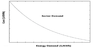
Also we can see the negative slope of the demand which limits the ability of the monopolist to benefit from its power of market.
3. Theoretical foundation. Main theoretical guidelines of the tools used
In [4], the demand curve in the distribution segment establishes the supply-demand balance based on certain characteristics of the natural monopoly, defining an equilibrium considered ideal and without influences from externalities that lead to a deviation from the optimum proposed in the economic theory. These externalities of technical characteristics have their origin in the components of the electrical system and make up the energy losses that must be measured and it controlled to reduce damage to the environment. These losses are generally classified as:
Technical losses: occur due to physical causes like to the circulation of the electric current and the voltage in the networks. This combination is known as the Joule effect.
Non-technical losses: it refers to the effective energy supplied but not measured (EESNM) or not commercially registered. The causes that originate this EESNM and according to the objective of this work, can be subclassified as follows:
- Losses due to theft: includes energy that is illegally appropriated from the networks by users through clandestine connections. They do not have measuring devices.
- Losses due to fraud: corresponds to those users who manipulate the measuring devices so that they register consumption lower than the real one.
- Losses due to administration: it refers to energy badly registered administratively by the company; due to measurement errors in the electrical connection of the users; incorrect registration due to meter obsolescence; incorrect measurement in public lighting installations.
3.1. Current regulatory context and the influence of non-technical losses on the main technical-economic parameters
The current context from the legislative and normative point of view is developed through a regulatory mechanism. By that previous, it is created a specific sector where distribution companies (mostly natural monopolies) and organisms called regulatory entities are related, with a distinctive characteristic, each one has its own autonomy and legal conditions.
The regulatory structure [8], is centralized at the National level through a organism called National Electricity Regulatory Entity (NERE), which has its representation in each province by organisms called Provincial Electricity Regulatory Entities (PERE). These entities allow each province has a contract (Concession Contract) where equitable values are agreed for both parties in terms of the energy purchase price; investment plan and its associated costs; total losses; taxes; all this included and weighted within of parameter called the quality of service
Currently in distribution, the total electrical losses can be defined from an energy balance, as the difference between the energy input (purchase) and the energy output (sale) referred to the complete system. The numerical value obtained represents the total losses that includes both technical and non-technical losses, which formula is shown below:

Where TL: Total Losses.
TechL: Technical Losses.
NTechL: Non Technical Losses.
Once the energy balance has been carried out, the non-technical losses are determined as the difference between the total losses and the technical losses, both conveniently measured. Eq. (1), allows the distribution company to quantify non-technical losses as a percentage of total losses, generating an economic deficiency. The direct influence of the above on a parameter called Distribution Added Value (DAV), which analytically characterizes technical losses and approximately non-technical ones imply an incomplete treatment of the subject.
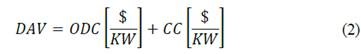
The Distribution Added Value is made up of two components:
The Own Distribution Cost (ODC) in this work, is developed “ceteris paribus” and as a function of the non-technical losses associated with parameters considered traditional.
The Commercial Costs (CC), present the particularity that due to their varied nature, they can reflect a different origin within the company, leading to incorrect imputations. In this article they are only mentioned leaving the development for future work.
The following formula allows us to know the existence of two components of the costs affected by the total losses:
The proposed methodology will weight the non-technical losses based on variables currently used to control the operation of the system; the current profile and the voltage drop adapted to the use of artificial intelligence techniques, will allow the desired quantification. Its introduction in eq. (2) will allow to establish its influence on the quality of the service.
4. Classification and identification of the origin of non-technical losses
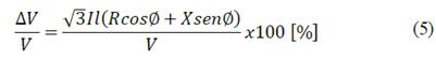
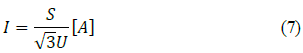
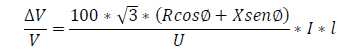
As mentioned above, the application of the currently existing parameters will allow a systematic analysis of non-technical losses. Due to the absence of variables that directly quantify them, a possible solution is to study percentage parameters that have a variation behavior in patterns or sets of values that allow them to be described. One of the parameters chosen is the percentage of voltage drop. The calculation procedure accepted by current regulations to determine it in three-phase systems uses the following equation:
If the parameters of ohmic resistances or reactances are referred to in the distribution lines with respect to units of length, to take into account their influence on the voltage variation, eq. (3) can be expressed as:

Where l: length in [Km].
R: resistence in [Ω/Km].
X: reactance in [Ω/Km].
The voltage drop will depend on the construction of a current profile that it is a direct function of demand, therefore, a measurable parameter. If we can consider eq. (4) as a fraction of the nominal voltage, we get:

By identifying current patterns with a neural network to calculate their magnitude using eq. (5), we can determine the percentage of voltage drop. The resulting dimensionless variable, expressed in% of the relationship between the voltage variation and its nominal value indirectly represents the non-technical losses (NTechL).
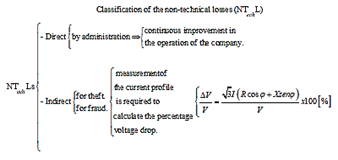
The proposal is to classify NTechL into direct and indirect, where the first are intrinsic and specific to the company, so they are under the exclusive control of the organization, while the indirect ones are those analyzed because they have a negative influence distribution system. Therefore, its quantification is important to obtain a stochastic profile of a phenomenon that is difficult to identify and affects the company.
Chart (1) summarizes the proposed classification for the control and quantification of NTecLs. The demand measurement allows to determine a current profile that it will applied to organize the percentage drop in voltage in defined patterns and classify them within limit values. Failure to comply with the imposed conditions causes a network review.
4.1 Non-supplied energy measurement methods
In [6] Economically Adapted Electric Distribution Systems (EAEDS) are described, in [7] the cost of Non-Supplied Electric Energy (NSEE) based on rules is defined without methodological fundaments. However, for the purposes of this work, if an adaptation of the regulation mechanism applied to the electric power distribution segment is carried out [8], where the NSEE will be expressed in terms of the NTecLs, the result will be an inefficiency indicator in terms of quality service from a probabilistic sample, precise enough to identify deviations from the values considered as reference. With this function, the company will have a diagnosis of possible penalties, before to submitting annual reports to the regulatory organism. Therefore, it is necessary to use control methods that can be of two types:
Control at the point of supply.
Energy balance by zones.
Despite the benefits of applying control at the point of supply, the effectiveness of the procedure can be optimized by applying Energy balance by zones.
4.2 Description of the energy balance method
The use of energy recorders to carry out the input-output balance at one point, will allows obtaining the current profile from the energy difference.
The use of energy recorders, preferably profilers, will allow from an energy input-output balance at a point, to obtain the current profile by calculating the net energy. The advantage of the Balance of Energy method over the control method at the point of supply is that the profile of the energy consumed in the sector is obtained at regular time intervals in a simpler way. In this way, the characteristics of the sector will be known from the record of maximum demand, a parameter that in addition to detecting energy losses (although they would not be significant in quantity), would allow the determination of excessive levels in the power contracted by users by inspection.
The method is applied at different levels of the network:
a) From the transformer or low voltage distribution center.
b) In a section or sector of the distribution network.
c) At the point of supply.
d) Next to the user's meter.
This work will only use the first two modalities, stating that the obtaining and selection of patterns carried out by the neural network will arise from the correction or update of the error matrix in each iteration. These are described below.
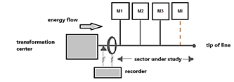
a. Energy balance from the transformer
This energy balance method is characterized by its simplicity of application; it consists of installing a recorder energy on each low voltage output of the power transformer as shown in Fig. 3 or on small power boards. During a few days or weeks, the total energy is recorded and compared with the energy pattern obtained by a neural network installed at a specific point in the sector. By comparing between the energy accumulated in the users' meter devices and to the energy billed, the method allows the detection of the magnitude of energy loss in the area
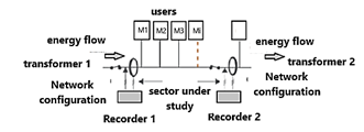
b. Energy balance in a sector of the distribution network
In areas with high demand there is more than one low voltage distribution center, therefore the energy balance should be carried out by sections delimited in switching points or "network division". Successful measurement will require the use of two measurement equipment capable of recording energy in both directions (“in” or “out” flow measurement), as shown in Fig. 4.
During the registration period (for example: 1 month), contingencies may occur in the network that force to modify the usual configuration (transitory state of the network during the duration of the contingency called altered configuration), producing a change in the direction of the Flow in the network. The recorder (profiler / totalizer) will detect the direction of the energy flow and indicate how much energy was counted in each direction, allowing the amount actually consumed in the area to be determined. With this technique, a multiple comparison alternative is available, the registered energy is compared with the sum of the readings in the energy meters, data processed by the neural network.
5. Description of the neural network.
The differential treatment of the topic related to NTechLs is found in the calculation and determination of the error matrix that depends on the operation of a neural network (NN). According to bibliographies consulted in the references, it was concluded that there is no method that allows determining the optimal number of hidden neurons to solve a specific problem, so most of the simulations are determined by trial and error, reason by which the use of the first derivation of the Widrow-Hoff rule of stochastic approximation is proposed. In reference [3], this concept is developed, mentioning to the author that the stochastic approach is used to solve non-linear problems whose variables present some dispersion, this constitutes another distinctive element in a sector that actually considers linear phenomena. In order not to extend into theoretical developments, the neural network concept is based on [1], using a multilayer perceptron neural network (MLP) obtained from adding hidden layers to the simple perceptron. This architecture is usually trained with the algorithm called error backpropagation or BP or by making use of some of its variants. The set of MLP architecture + BP learning is often called a backpropagation (BP) network.
The neural network programmed with the MATLAB software does not use the code included by default in the program, it is a .m code created to process the necessary data and has the appearance shown in Fig. 5.
5.1 Choise of the criterion
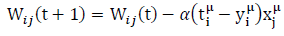
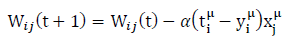
Without despice the concept of error and at the same time reducing the dispersion of the variables in the simulation results, it was decided that the NN works under the criterion of the first derivation of the Widrow-Hoff rule of stochastic approximation whose theoretical development in [2] allows to arrive at the error formula given below and used by the algorithm:

Where Wij (t+1) is the update matrix of synaptic weights; Wij (t) is the matrix of synaptic weight obtained in the previous iteration; α is the learning rate of the network; tµi is the vector representing desired output for the i-th neuron in the output layer according to the patterns presented in the input; yµi is the vector representing the output obtained in the i-th neuron of the output layer according to the patterns presented in the input; Xµi is the vector representing the input of the patterns in the jth neuron of the input layer.
5.2. Learning process
The NN learning process has the classic characteristics of the methodology proposed by the consulted bibliographies and the randomness in the input patterns that the trainable device must deal with according to the following steps:
1. Network weights and thresholds are randomly initialized with values around zero. The stochastic approximation method used is modified so that the threshold values are an additional weight, with a constant value equal to -1, thus simplifying the process of updating the synaptic weights.
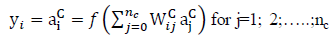
2. Presentation of the input patterns of the set of variables to be analyzed, weighting them and propagation towards the output of the network as follows:
a) Activation of the input neurons of the input layer

So
ai = xµi for j=1; 2;…..;n that is to say:

b) Activation of hidden layer neurons C (aic)
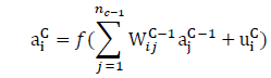
for i=1; 2;…..;nC y C=2; 3;….;C-1
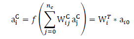
threshold values uci are considered as an additional weight as follows: associating the j-th element equal to zero with the threshold function with a value equal to -1, that is for j=0; wi0 =xi y x0 the formula reduces to
1. When the data passes through the hidden layer, the output layer is activated where the propagation from input to output is done in two parts; first using the stochastic gradient descent or forward propagation technique; then back propagation updating synaptic weights and polarizing them
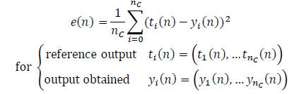
1 Once the output is obtained, the mean square error committed by the network for pattern n is evaluated using the following equation:
2 The first derivation of the Widrow-Hoff rule of stochastic approximation is applied
For modify the weights and thresholds of the network.
1. Steps 2, 3 and 4 are repeated for all training patterns completing a learning cycle.
2. The total error E or error made by the network, is also known as the training error is evaluated with the equation:
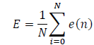
Where E is calculated using the training patterns.
1. Steps 2; 3; 4; 5; 6 and 7 are repeated until reaching a minimum in the training error after m learning cycles. For the case analyzed, a value of m = 100 was considered.
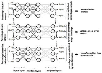
5.3 Input patterns
The neural network (NN) applied in a part of an electrical distribution system receives the energy reading from the network, from that information it calculates the following patterns that must be processed simultaneously.
- Percentage inputs current.
- Percentage drop in voltage.
- Percentage losses due to transformation.
These patterns are different magnitudes, with different units but its influence the system is the same, which is why each one is weighted to be able to train the NN and achieve their optimization. With these results, an analysis of the load center of the distribution circuit is carried out, which will once again allow the NN to process the updated information to obtain optimization in the second instance.
6. Non-technical losses calculations. Presentation of the context
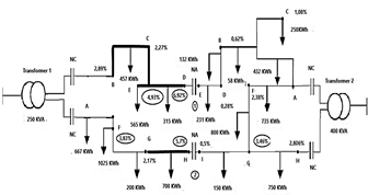
The closed low voltage system or mesh configuration used for the analysis; simulation and optimization of non-technical losses, has a nominal voltage of 0.4 KV and is made up of two Control Areas. We will call Control Area 1 the circuit whose energy comes from transformer 1 with nominal power of 250 KVA, analogously, Control Area 2 is the circuit energized from transformer 2 whose nominal power is 400 KVA. These areas are connected to different medium voltage lines with a nominal voltage of 13.2 KV. The simplification of the study is achieved with an equivalent circuit shown in Fig. 6, formed by both transformers and substituting the distributed demand for an effective concentrated demand. The system can operate from both areas through two low voltage power disconnectors 1 and 2.
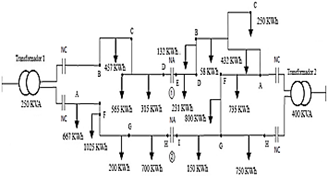
The proposed configuration is predominant in the study area (Concepción del Uruguay, Entre Ríos Province), it is the one selected because it allows isolating faults; restore power flow within minutes by reducing NSEE due to random events; a decrease in the frequency of cuts is achieved. In case of maintenance work, transient parallels can be carried out, for which it is important that the sequence of phases and the direction of the currents are the same in both sectors. Controlling these parameters that define the quality of service, penalties are also minimized. Therefore, points 1 and 2 are critical and must be under strict observation free of errors.The analysis of the numerous data difficult to control given the nature of electrical energy, whose instantaneous supply according to demand requires a continuous control in real time, leads to the purpose of an instantaneous verification if the supplied energy program is respected and taking immediately take the necessary actions to correct deviations that arise (increase or decrease in demand), always seeking to minimize operating costs and maximize supply reliability. The application of neural networks that control the state variables in points 1 and 2; considering the distributed demand in the sector compensated by phase and then reducing it to a concentrated demand at points determined by the voltage drop parameter, it will allow the system to be reconfigured in a theoretical and practical way to achieve energy efficiency.
6.1 First calculations
The demand values are obtained by two energy recorder connected as in Fig. 4. Initially, the NN calculates the nominal current of the transformer whose power is known:
The distributed demand in the sectors and for the purposes of this work called Effective Demand of the Sector (DES in spanish) is structured in a matrix form.
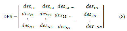
Eq. (8) Generalized as follows
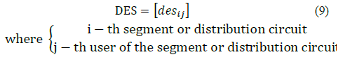
The parameter desij represents the effective unit demand of the user measured in [kWh] whose geographic location is determined by coordinates in degrees; minutes and seconds of latitude φ[º ´ ´´ ] and longitude λ [ º ´ ´´ ]; it also contains real information on the harmonics of the network where the 3rd and 5th are currently used to determine the Total Harmonic Distortion (THD).
The distance from the users to the recorders related to the length of lines, originates the effective length (LE in spanih) and in matrix form:
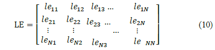
Eq. (10) Generalized as follows:
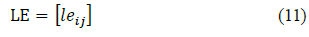
leij is the unit effective distance with units of [km], considered in this way to make it compatible with the electrical and magnetic parameters of R and X given in [Ω / km] and measured by coordinate differences converted to length.
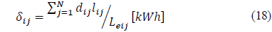
Multiplying the matrix from eq. 8 and its homonymous transpose from eq. 10
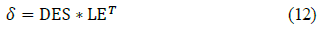
Numerically δ it is a quantity of energy per distance [kWh-km], This variable is created to discretize the energy demanded in the segments whose locations are punctual. This previous step will make it possible to obtain the concentrated demand, an important parameter and basis for sending patterns to the NN.
For example, for segment 1:
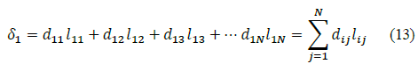
where i= 1; 2; 3;…N
To determine the point of application of the load, we use eq. 5 and the definition of three-phase effective demand. If we adapt the demand equation so that it adjusts to the conditions imposed by the quality of the service:

From eq. 14, the magnitude U within what is imposed by the quality of service must be kept constant with a dispersion of  1,73 due to the fact that by the disposition of the energy recorders the total energy measured is considered. Then, a parameter is defined that we will call χ or validation of the efficiency of the service, since a variation of the factors that integrate it outside the allowed dispersions will serve as a warning for the NN that will contemplate it within the pattern selection process. In equation form:
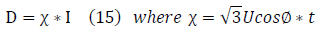
In eq. 14, D is the state variable of the problem; χ is a non-linear factor representative of the quality of the service and I is a control variable.
Eq. 5 is algebraically adapted to the problem as follows:
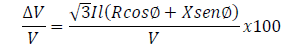
The parameters conditioned by current regulations can be modified according to criterion follow:
It can be simplified the equation as follows:
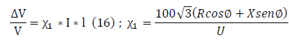
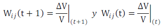
Eq. 16, is important because imposes a restriction criterion since ∆V⁄V is a bounded state variable with tolerance≤3%; χ1 is another non-linear factor which represent quality of service and condition of lines; I is a control variable. Established the conditions and using eq. 6 of point 5.1
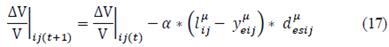
The distance or point of application of the concentrated load can be determined, based on the calculation of the error matrix of the voltage drop that is used at the beginning of the algorithm, where:
where:
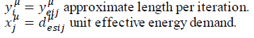
ti μ=lij μ reference length.
The α factor or learning factor, is modified considering within it the demand and total length of the lines, the information available from the energy loggers and the inspection of the system. So, the factor α = ς * 1 / δ is obtained, where ς comes from the function MATLAB rand that returns real numbers between 0 and 1 that are drawn from a uniform distribution and ς is obtained from eq. 12.
The Widrow-Hoff rule of stochastic approximation modified for the determination of error matrix of the voltage drop is:
When  ;where m =100 by previous mention in point 5.2, then from eq.17
  is obtained as the location of the concentrated demand referred to distance from the transformer and whose value is quotient between eq. 13 and Leij.
General equation
allows to obtain each one of the concentrated demands for the distribution sector under study. The neural network analyzes each input pattern or concentrated demand received; computes the actual currents and performs initial weighting in the traditional way, then uses the Widrow-Hoff rule of stochastic approximation to compute the error matrix.

Where Eij (t+1) is the updated value of the error for each iteration; Xµ
j is the input in [A] obtained from the service efficiency validation parameter χ in eq.15 and δi
j of eq
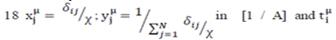 in [1 / A] and tµ
i referent output.
in [1 / A] and tµ
i referent output.
For this example, the concentrated loads are applied at seven points in the system. In this way, the same amount of current values are obtained, the sum is compared with the nominal current of the transformer and in case of an excessive value, the device generates an alert automatically calculating approximate values of weighted currents in the first instance. The neural network analyzes each point of concentration of the demand. The users are actually distributed by sections and the trainable device proces them as simple input patterns.
The Table 1 shows the results obtained in the simulation carried out by the trainable device with respect to the first set of patterns presented.
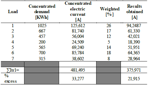
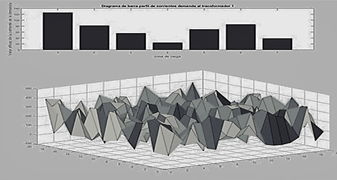
The Table 1 shows the results obtained in the simulation carried out by the trainable device with respect to the first set of patterns presented. The results obtained show that at the beginning of the network study there is an excess load of 33.27784%, reducing to 21.91578% in the first approximation. In Fig. 7 the bar and matrix diagrams constitute the first stochastic approximation of a non-linear situation. The current profile is a trend of all individual consumption patterns; it shows an unbalanced demand whose real aspect would be a discrete sequence. In the matrix diagram, the optimal value is difficult to identify due to the existence of peaks and valleys. Here is the efficiency contribution of a spectral analysis using the first derivation of the Widrow-Hoff rule of stochastic approximation and superiority with respect to a linear analysis
6.2 Voltage drop optimization calculations
For the case of voltage drops in areas of high load density such as the one proposed where there are more than one low voltage distribution center, eq. (17) will allow the identification of compromised areas. Fig. 8 shows the result obtained by the NN as a function of the characteristics of the conductors.
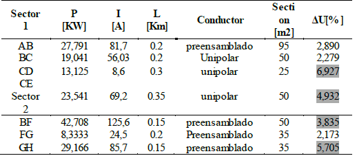
With all the before mentioned data, the trainable device adjusts to the voltage drop calculations in accordance with current regulations and detects the sections where the voltage drop percentage has high values, as shown in Table 2
how a statistical complement, in Fig. 9 the voltage drop profile is detailed.
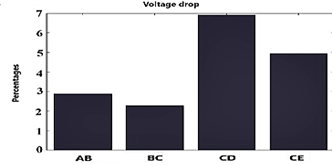
6.3 Comparison of currents vs voltage drop
Once the magnitudes were calculated and the profile established, the NN compares both using the Kolmogorov-Smirnov test (not developed in this work) to establish the association between the results and the geographical location where the percentage values out-of-norm detected. For the example, the bar chart in Fig. 9 shows that the CD segment has a high value. From Table 1, this segment corresponds to the current values I5 and I7 produced by the concentrated demands of 565 KWh and 315 KWh respectively. In reality, the CD segment is made up of a total of 41 users who have been identified by phase and distributed consumptions.
The bar chart in Fig. 7 contains the profile of currents calculated from the concentrated loads, which are associated with a discrete sequence of consumption per user shown in Fig. 10.
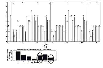
From the observation of both graphs it can be inferred that from the selection of patterns, there are three maximum values of 8 A approximately that exceed the contracted power values and other values that oscillate between 5 A and 6 A. In this way, a limited interval is established  where the mean value considered by the Neural Network for the selection of patterns is approximately 6.5 A. From the before mentioned interval, the values 5 A are selectable; 6 A and 8A as potential candidates to detect the possible alteration of the supply points, which is verified by comparing with the percentage drop in voltage in the DC section, which amounts to a value of 6.92% at the point where the system is installed. Trainable device and normally open low voltage load-breaker.
7. Conclusions
This work in principle exposes the inexistence of an adequate methodology to quantify non-technical losses (NTechL) of an electric service company. In line with current legislation that considers companies as natural monopolies, they are regulated by regulatory mechanisms, which lead to generalizations regarding the determination of important parameters that influence the operation; expansion and costs of organizations. There is no doubt that non-technical losses treated incorrectly from the technical point of view, would impact the legislative, possibly resulting in a normative transformation, which would generate a drastic change of paradigm with the consequent increase in associated costs, which without proper identification would directly affect the quality and price of the service. The proposal of the use of artificial intelligence to carry out a parameterization of non-technical losses using a neural network, which selects patterns of currents and voltage drop; compares them and considers them as possible candidates to represent some type of alteration when they oscillate within a range calculated and determined by the device, it allows the specific quantification of these losses, so within the current context the contribution of this tool is to provide precision within the limits imposed by regulations constituting a modern shape; different from analyzing and simulating data, incorporating into its operation the biases due to non-linearity, such as the parameter, which is increasingly influential in the electricity service and that if not properly considered would affect efficiency in the short and medium term of the cost structure of electric power distribution systems.

