


 Inglês (pdf)
 Artigo em XML
 Referências do artigo
 Enviar este artigo por email
 Citado por SciELO
  Citado por Google
  Similares em
SciELO
Similares em
SciELO  Similares em Google
 Permalink
Introduction
Exploration industries commonly use seismic imaging tools, which allow waves to propagate through subsurface rock structure and reveal possible crude oil and natural gas bearing formations. First arrival traveltime tomography is a classical seismic imaging method that for many years has proven to be stable, gives good results, even in lateral heterogeneous media (Chabert, 2010). The data set for the inversion is small (consisting only first arrival travel times), so the method is fast and efficient. However, the first arrival travel times are only sensitive to the long wavelengths of the medium (Chabert, 2010) which limits the possible resolution of the final estimated model. Another disadvantage of the method is the picking of the first arrivals from the seismic data, which is both time consuming, and introduces the possibility of picking errors (Improta et al., 2002). On the other hand, FWI, uses amplitude, travel time and phase information simultaneously to invert the model parameters. FWI is an inverse method that generally employ the least squares objective function to minimize the difference between observed seismic data and synthetic seismic gathers by updating the initial model parameters until convergence (Margrave et al., 2011). The model updates are generated by reverse time migration of the data residual.
The main obstacles that have prevented FWI's common application in exploration seismology are its computational cost and need for a good initial model (Ma, 2010). Various efforts from different perspectives have been developed to reduce the computational costs associated with gradient computation and seismic data generation. For example, Sirgue and Pratt (2004) and Operto et al. (2007) limited the number of frequencies in updating the model. Vigh and Starr (2008) used plane wave method for three-dimensional problems and Margrave et al. (2010) used Phase Shift Plus Interpolation one-way wave gradient calculations.
In this study, FWISIMAT is developed in both time and frequency domain based on acoustic wave equation. The frequency-domain inversion approach is equivalent to the time-domain inversion approach if all of the frequency data components are used in the inversion process (Hu et al., 2009). FWISIMAT use Non-Linear Conjugate Gradient (NLCG) (Dai and Yuan, 1999; Hanger and Zhang, 2005) and Broyden-Fletcher-Glodfarb-Shanno (BFGS) optimization procedure in time and frequency domain algorithms respectively. As to the forward modelling, second order finite difference method is employed due to its high efficiency. This discretization scheme includes absorbing boundary conditions applied on the edges of the velocity medium. However, in order to initiate any iterative scheme an initial model is required (Kanli, 2009), and is derived from smoothing the true velocity model using a Gaussian kernel.
2. FWISIMAT for Time Domain
Full Waveform Inversion is an iterative minimization technique to update the initial model parameters, which is described at kth iteration as follows:

where, m is the model parameter, P is the direction of update and α is the step length.
FWI is composed of forward modelling computation, gradient computation, and valid optimization technique (Cao and Liao, 2013)
2.1 Forward Modelling
Forward modelling is a necessary step for solving any inverse problem. The governing equation for time domain FWI is non-homogeneous 2D acoustic wave equation (Eq. 2).

In Equation 2, u(x, z, t) is the source wave-field, v(x, z, t) is the velocity, f(t) is the source time function and (x s , z s ) is the source location in space.
Let u l n m be the wave-field at the time l∆t and spatial position (n∆x, m∆z), v nm be the velocity at (n∆x, m∆z) then Equation 2 can be discretized using central difference scheme as follows:
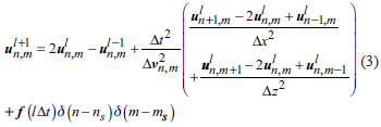
with the initial conditions

The numerical stability conditions for Equations 3 and 4 is as follows:

The unsuitable choice of time and spatial steps may cause severe dispersion and wave distortion in wave simulation. In order to suppress numerical dispersion, it is usually required that there are 10 sampling points per wavelength in Equation 2,
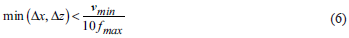
For the same frequency, the numerical dispersion increases as the spatial steps increase. However, the dispersion can be depressed if the higher point approximation schemes are used.
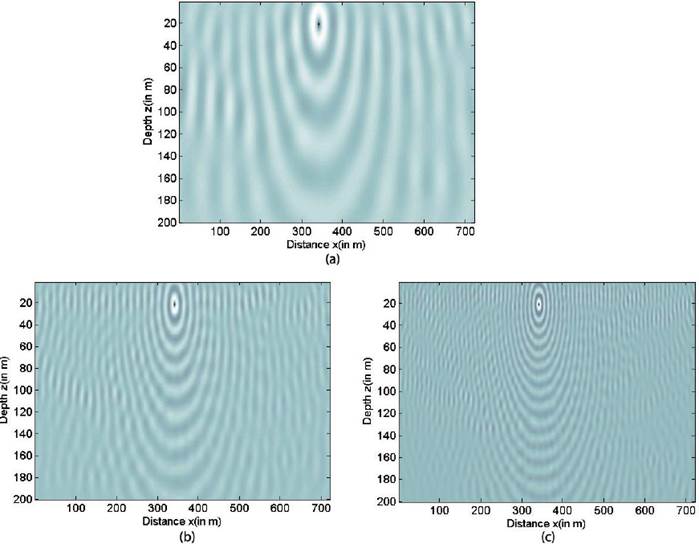
In numerical computations, the computational domain is usually truncated to a finite region. So, absorbing boundary conditions (ABCs) are included in order to reduce reflection from the edges of the grid. The absorbing boundary conditions are constructed from paraxial approximations of the wave equation (Clayton and Enquist, 1977). Figure 1 illustrates the effect of boundary conditions when the wave-field hits the edges of the medium. Wave-fields are recorded for each time at each receiver positions per source. These records are called as synthetic seismograms (Fig. 2).
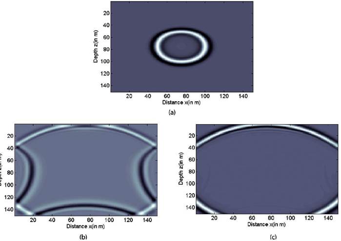
Figure 1 Effect of boundary conditions, (a) Wave-field at time 0.17 sec, (b) wave-field at time t = 0.42 sec (no boundary condition is used), (c) wave-field at time t = 0.42 sec (absorbing boundary conditions is used).

2.2 Gradient Computation: Reverse Time Migration
The objective function (O(v)) that would be minimized is given as follows:

where, d obs is the observed data and d cal is the calculated data. The gradient of the objective function is given as follows:

where, q s represents the back-propagated wave-field from receivers to source. q s can be computed from Equation 9 backward in time (Demanet, 2015).
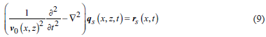
In Equation 9, r is the residual field (Eq. 10).

The sum over in Equation 10 is sometimes called a stack (Fig. 3). Stack uses the redundancy in the data to bring out the information and reveal more details (Demanet, 2015).
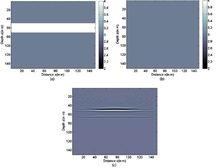
Figure 3 An example of gradient computation using reverse time migration method, where (a) is a theoretical model (b) is initial model and (c) is migrated image.
A systematic way for solving back-propagated wave-field (Eq. 9) is to follow the following sequence of three steps: (1) time reverse the data residual r (x, f) at each receiver position, (2) solve the wave equation forward in time with this new right hand side, and (3) time reverse the result at each receiver position in x.
2.3 Optimization: Non-Linear Conjugate Gradient Method
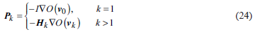
Conjugate gradient optimization method updates the velocity model according to the descent direction P k (Eq. 11).

According to Pica et al., (1990) step length is estimated as follows:

where, J k stands for Jacobian matrix and […] denotes inner product.
For computing the direction P k , NLCG optimization process is used (Hanger and Zhang, 2005), which decreases the objective function along the conjugate gradient direction (Eq. 13).

In Equation 13, γ k γk is computed according to Equation 14
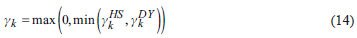
in which

This provides an automatic direction reset while over-correction of Y k in conjugate gradient iterations. It reduces to steepest descent method when the subsequent search directions lose conjugacy.
2.4 Numerical Computation: Marmousi Velocity Model
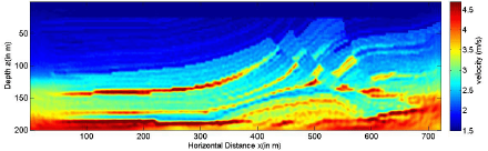
The Marmousi Velocity model is a benchmark model for testing the ability of migration or inversion methods (Zhang, 2009). The original velocity model is shown in Figure 4. However, for this study a resampled velocity model (true velocity model) is used as illustrated in Figure 5.

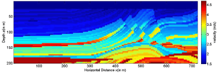
The Initial model is generated by smoothing the true model using a Gaussian kernel (Fig. 6).

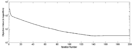
There were total 31 sources at a depth of 10-m and 720 receivers at a depth of 2-m equally spaced in the medium. Absorbing boundary condition is applied over all four edges of the medium. Grid spacing is kept at ∆x (=∆z) =0.01-m, sampling is taken over At = 0.0014 with number of sample point set as Nt=890. To save computational, we use the whole frequency band (0-20Hz) for the inversion (in frequency domain, this implementation is different). In practice, multiscaling approach is employed to reconstruct the model from low to high frequency fashion (as discussed later in the paper). This implementation generally cause the difference of the resolution in different inversion algorithms. However, the time-domain FWI is still able to provide good estimation of the acoustic parameter without sacrificing the high resolution. Figure 7 and Figure 8 represent the inversion result after 200 iterations and the value of the objective function after each iteration.

A more qualified analysis of the velocities is easier when looking at the velocity profiles in Fig. 9. Velocity logs at three different locations are extracted (at 200, 400 and 600 m) from true, initial and final model. In all three logs, the final velocities from FWI result matches with the true velocities very well.

3. FWISIMAT in Frequency Domain
Frequency domain Waveform Inversion, which includes solving the wave equation forward modelling and inversion, is similar to time domain waveform inversion. The efficiency of frequency domain FWI depends on the number of frequencies used for the inversion and is independent of the number of sources used for inversion.
3.1 ForwardModelling
For frequency domain forward modelling Equation 2 must be converted into frequency domain (Eq. 16).
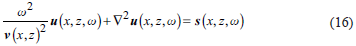
In Equation 16, ω is the frequency, ν (x, z) is the velocity in the medium, u (x, z, ω) is the source wave-field, and s (x, z, ω) is source in freuency domain (Fourier-transform of time-domain source wavelet). The boundary condition in frequency domain is given as follows:

where, nn is the outward normal of the boundary, h = ω / ν (x, z), and i is the imaginary unit (Erlangga, 2008; Zhang and Dai, 2013). By means of the finite difference technology along with the boundary condition, the wave equation (Eq. 16 and 17) can be recast into matrix form as follows:

In Equation 18, A is a complex-valued, nx x nz (discretization along xx and z direction) order impedance matrix and it depends on frequency, medium properties, finite difference format, and boundary conditions (Wang et al., 2012). Solving the linear system in Equation 18 wave-field can be obtained (Fig. 10). Wave-fields are recorded for each frequency at each receiver positions per source. In FWISIMAT the above mentioned process is implementation as follows:

In Equation 19, D (= d cal ) is the matrix inversion operator and r' is the transpose of the vector consisting receivers at spatial positions and Q is the source vector. Figure 11 illustrate the data obtained from a same source but for different frequencies.
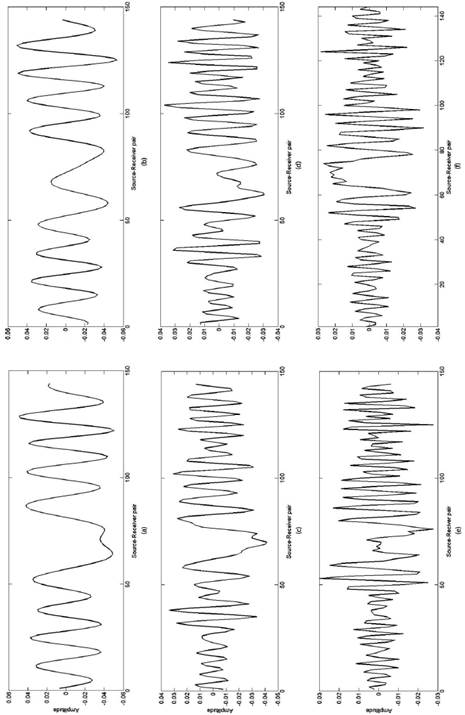
Figure 11 Frequency data for true model at, (a) 5 Hz frequency component, real (b) 5 Hz frequency component, imaginary (c) 12 Hz frequency component, real (d) 12 Hz frequency component, imaginary (e) 20 Hz frequency component, real (f) 20 Hz frequency component, imaginary
3.2 Gradient Computation: Reverse Time Migration
The gradient of the objective function in frequency domain is given as follows,
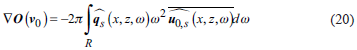
where,  represent the complex conjugate operator (Demanent, 2015). The integral in o in above equation is over R and should be truncated to the number of frequencies used in the process. Equation 20 represents the frequency domain version of Equation 10. In FWISIMAT the back-propagated wave-field
  is computed as follows:

where, V  is back-propagated wave-field. Dobs can be obtained from Equation 19 if applied on true model.
Optimization: Broyden-Fletcher-Goldfarb-Shanno (BFGS)
In time domain FWI, NLCG optimization method is used. NLCG consumes a substantial time to converge. According to Zhang and Luo (2013), the BFGS based method has higher inversion accuracy and converge faster than the conjugate gradient based algorithm because the later uses the second order derivative information in computation.
The BFGS method is a quasi-Newton method which proposed dependently by Broyden (1970), Fletcher (1970), Goldfarb (1970), Shanno (1970). Let H k is the inverse hessian approximation then the next iterate will be given as follows:

where, b k = m k+1 - m k and g k = ▽O(m k+1 ) - ▽O(m k ). For k = 1, H 1₺33▽▽ can be approximated by an identity matrix. The next update on the model parameter is given as follows:

where,
BFGS method does not require exact line search in order to converge, therefore, Wolfe line search algorithm (Wolfe, 1969; 1971) is acquired to find step length αk. The strong Wolfe line search algorithm requires the following conditions to be satisfied.
In Equation 26 0 < q < C2 < 1.
Numerical Computation: Marmousi Velocity Model
True and initial velocity model for frequency domain FWISIMAT are kept same as Figure 5 and Figure 6 respectively (ensuring 10 grid-points per wavelength). The number of sources and receivers are 30 and 90 which are equally spaced in the medium at a depth of 20-m. The absorbing boundary conditions are applied on all edges of the medium. The inversion result after 25 iterations is shown in Figure 12. The inversion is from low to high frequency, and choice of which is usually related to the model. The low frequencies are more linear related to the model perturbations than the high frequencies (Sirgue, 2003). Therefore, the inversion process should start with the low frequency components and progressively add higher frequencies. This will help mitigate some of the non-linearity of the problem, hence increasing the chances of finding the global minimum. It also ensures that progressively higher wavenumbers are recovered (Ravaut et al., 2004).
According to the experience and experiments, twelve frequencies are selected, not only to obtain good results, but also for faster computation. The twelve frequencies from low towards high are 1.00 2.73 4.45 6.18 7.91 9.64 11.36 13.09 14.82 16.55 18.27 20.00. Figure 13 shows the objective function value in logarithmic scale during the inversion process.

Figure 14 shows the velocity comparison among the final, true model and initial model at different horizontal distances. After frequency domain waveform inversion algorithm, the final result is obtained close to the true velocity model, especially that the near-surface speed is almost identical to the theoretical model. The results confirm the validity of the algorithm.

4. Conclusions
The Full Waveform Inversion method and its capabilities, when applied to a complex geological model, have been presented in this study. The FWISIMAT algorithm used in the study, performs an iterative search for a velocity model that minimizes the residuals between the data computed in the velocity model and the observed data, i.e. the final result is a "best fit" model. The whole wave-field, including both waveform and phase, is being used as data. FWISIMAT computes in the time and frequency domain. Comparing with the frequency domain inversion method, the time domain method has the advantage of high efficiency in forward modelling as the wave modelling in frequency domain requires solving a large-scale system at each iteration which is time consuming for large scale problems. Apart from this, time domain modelling provides the most flexible framework to apply time windowing of arbitrary geometry. In the frequency domain, the computational cost is only proportional to the number of frequencies used in the inversion, and not the number of sources. If the seismic data contains wide angle components, there will be a redundancy in the wave number spectrum present in the data, such a redundancy can be exploited in the frequency domain FWI by inverting fewer frequencies (and hence save computational costs) because it is possible to invert for single, discrete frequencies one at the time. Another great advantage with the frequency domain implementation is the ease and efficiency when adding multiple sources. The method is very sensitive to the non-linearity of the problem, and proper input parameters, such as an accurate starting model and an initial frequency as low as possible, is important for obtaining optimum results. In this work, it is shown that Full Waveform inversion has a great potential for estimating complex velocity models such as Marmousi Velocity Model when the acquisition parameters are as optimal as possible. For the future, applying FWI to real data from more complex geological medium and developing a migration tool and test the effect of FWI on a migrated image, are interesting challenges.

