


 English (pdf)
 Article in xml format
 Article references
 Send this article by e-mail
 Cited by SciELO
  Cited by Google
  Similars in
SciELO
Similars in
SciELO  Similars in Google
 Permalink
Introduction
It is well known that the production frontier and technical efficiency anal yses on a productive unit assume that deviations of the observed product from its maximum (or potential) attainable output, located on the produc tion frontier, are due exclusively to inefficiencies of the productive unit (see, e.g., Kumbhakar & Lovell, 2000; Coelli, et al., 2005). For instance, if the as sumed production function is a Cobb-Douglas technology y = x⊤ β + v, where y and x are the logarithms of the observed output and the input vec tor respectively, then the production frontier x⊤ β is deterministic, and v = y −x⊤ β corresponds to the production inefficiency. The lack of randomness in the production frontier of this kind of models does not correspond to the real economic life, where uncontrollable random production shocks occur commonly.
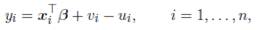
The stochastic frontier production model (Aigner, Lovell & Schmidt, 1977; Meeusen & van den Broeck, 1977) is specified as
 () 1
() 1
where yi is the observed output and xi the k-dimensional vector of inputs
for the ith firm, 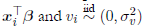 represent the deterministic and noise components of the frontier respectively, xi
⊤
β + vi
is the maximum output reached by the firm which constitutes the stochastic frontier, and ui
is the non-negative random technical inefficiency component (i.e., the amount by which the firm fails to achieve its optimum). A symmetric distribution, such as the normal distribution, is usually assumed for vi. It is also common to assume that vi
and ui
are independent, and that both errors are uncorre lated with xi
. Typically, the production function relies on a Cobb-Douglas, translog, or any other logarithmic production model log(yi)= xi
⊤
β + vi
- ui
, where the components of xi
are logarithms of inputs, its squares and cross products.
represent the deterministic and noise components of the frontier respectively, xi
⊤
β + vi
is the maximum output reached by the firm which constitutes the stochastic frontier, and ui
is the non-negative random technical inefficiency component (i.e., the amount by which the firm fails to achieve its optimum). A symmetric distribution, such as the normal distribution, is usually assumed for vi. It is also common to assume that vi
and ui
are independent, and that both errors are uncorre lated with xi
. Typically, the production function relies on a Cobb-Douglas, translog, or any other logarithmic production model log(yi)= xi
⊤
β + vi
- ui
, where the components of xi
are logarithms of inputs, its squares and cross products.
Most of the proposed stochastic frontier models in the literature differ mainly on the assumed probability distribution function for the inefficiency component u >= 0 in order to apply the maximum likelihood estimation method. In this regard, Kumbhakar and Lovell (2000), Coelli, et al. (2005), and Greene (2008) present an extensive literature about some distributions. Some instances are the half-normal model u ~ N+ (0,θ2 u), where N+ denotes the non-negative half-normal distribution (Aigner, Lovell & Schmidt, 1977); the exponential model u ~ Exp(λ), λ > 0 (Meeusen & van den Broeck, 1977; Aigner, Lovell & Schmidt, 1977); the gamma model u ~ Γ(λ, θ), λ > 0 and θ > 0 (Stevenson, 1980; Greene, 1980a; Greene, 1980b); and the truncated normal u ~ N+ (µu, σu 2) (Stevenson, 1980).
An issue with applications of stochastic frontier analysis emerges when inputs are highly correlated, from which the multicollinearity problem arises, leading to precision loss in estimates. This loss is also given by low input variability. In the presence of collinearity, it is known that: (i) separating the individual effects of each independent variable could be a difficult task; (ii) the precision loss is expressed in large estimated variances of estimates, and hence the parameters could be non-statistically significant; (iii) the esti mated coefficients can have incorrect signs and impossible magnitudes; and (iv) there are instability problems in the sense that small changes in obser vations, or eliminating an apparently insignificant variable, can produce large changes in estimates (see, e.g., Belsley, Kuh & Welsh, 1980; Fomby, Johnson & Hill, 1984; Groß, 2003). Therefore, it is clear that multicollinearity is a data-driven issue rather than a statistical one (Belsley, Kuh & Welsh, 1980), which can have harmful implications for the estimation of technology coeffi cients due to their relation with the scale returns generated by the production model.
Despite these drawbacks, a great extent of literature on stochastic fron tier analysis considers the multicollinearity problem as unimportant or uses a non-statistical solution. For example, Filippini, et al. (2008) exclude the input whose correlation with other inputs is quite high in order to prevent multicollinearity. Other studies sacrifice the advantages of flexible functional forms for the deterministic component due to the cost of statistically insignif icant estimates generated by unreliable parameter estimates resulting from lin ear dependencies between inputs (Kumbhakar & Lovell, 2000; Puig & Junoy, 2001; Filippini, 2008). Finally, others argue that, when technical inefficiency estimation is the main aim, multicollinearity is not necessarily a serious prob lem and the interpretation of estimates is secondary (Puig & Junoy, 2001). To the best of our knowledge, no theoretical research has been reported on studying both the stochastic frontier analysis and multicollinearity jointly.
In this paper, we propose a principal-component-based solution for mul ticollinearity in a stochastic frontier model. Basically, we use a re-paramete rization of the model in terms of all k principal components and restrict the corresponding coefficient vector to those principal components associated to the r < k nonzero eigenvalues. Finally, estimates of the original model are recovered. The solution permits a joint estimation of the technical effi ciency and parameters through this better specified model. Also, through a simulation experiment, the proposed estimator is shown to be consistent and has less mean square error with respect to the traditional stochastic frontier analysis.
The rest of the paper is organized as follows. In Section I., the solution is described, and its performance is studied by a Monte Carlo simulation ex periment in Section II. In Section III., an application with real data is carried out. Finally, some conclusions are given.
I. The principal component solution
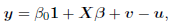
For the case where there is only near exact multicollinearity (i.e., when one or more nearly exact linear relations exist among the regressors), we consider the matrix representation of the stochastic frontier production model (1),
 () 2
() 2
where y, v, u, and 1 are n-dimensional vectors of observed outputs, produc tion and inefficiency random errors, and ones respectively; X is the n × k design matrix of inputs; and β the corresponding k-dimensional vector of coefficients. For clarity and notational simplicity, all inputs are assumed to be standardized in the sequel.
Now, based on the spectral decomposition of the k × k symmetric matrix X⊤X ,
X⊤X = P Λ P⊤ ,
where Λ = diag(λ1, λ2,..., λk) is the diagonal eigenvalues matrix (with λ1 ≥ λ2 ≥··· ≥ λk), and P =(p 1, p 2,...,pk ) the corresponding orthogonal eigenvectors matrix.
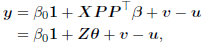
By the orthogonality of P (i.e., PP ⊤ = P ⊤ P = I), the regression model (2) can be re-parameterized as
 ()3
()3
where Z = XP = (z1, z2,..., zk) is the matrix of principal components zj = Xpj with the property zT j zj = λ j , ∀j, and θ = P ⊤ β.
From the theory of principal component analysis -PCA- (see, e.g., Jol liffe, 2002), it is well known that the principal components zj = Xpj are orthogonal, where the first principal component z1 has the maximal variance (i.e., the largest amount of information) of the original variables, the second principal component z2 has the next maximal variance after the first prin cipal component, and so on. Note that if the jth characteristic root λj is approximately equal to zero, then zj ≈ 0.
Additionally, if all k principal components are used, the same parameter vector β is obtained, which is unreliable under collinearity among the exoge nous variables as was pointed out in the introduction. In other words, fairly small eigenvalues of the
X⊤X
matrix generate imprecisions in the OLS esti mator  Therefore, the strategy consists in preventing that the estimate goes in directions λipj
associated to fairly small λj
(see Fomby, Johnson & Hill, 1984; Groß, 2003).
Therefore, the strategy consists in preventing that the estimate goes in directions λipj
associated to fairly small λj
(see Fomby, Johnson & Hill, 1984; Groß, 2003).
Thus, to deploy the strategy, we restrict β into the subspace spanned by the columns λ 1p1, λ 2p2,..., λrpr , where λ 1 ≥ λ 2 ≥ · ·· ≥ λ r > 0 are the r<k largest eigenvalues of X ⊤ X and λ r+1 ≈ λ r+2 ≈ ... ≈ λ k ≈ 0. This means that range ( X ) = r. Hence, in order to eliminate imprecisions, Massy (1965), Jolliffe (1982), Mason and Gunst (1985), and Hwang and Nettleton (2003) suggest using (i) the first principal components with the largest vari ance and highly correlated with output y, and (ii) those principal components of low variance but with high output correlation.
Therefore, the model (3) can be re-expressed using the subdivision of the eigenvalues into groups λ1 ≥ λ2 ≥··· ≥ λr > 0 and λr+1 ≈ λr+2 ≈ ··· ≈ λk ≈ 0 and defining the corresponding partition Z = (Z 1, Z 2) = (XP 1, XP 2), where Z1 is the n × r matrix with principal components as sociated to the nonzero eigenvalues and Z2 the n × (k − r) matrix with the rest of the principal components associated to the eigenvalues approximately equal to zero. Then, assuming that the first r principal components are highly correlated with y in order to simplify the notation, and using Z2 ≈ 0, the re parameterized model (3) can be expressed as
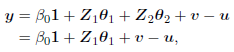
where θ = (θ1 T, θ2 T) T, with θ1 = P1 T β 1 and θ2 = P T 2 β 2. The constraint
Z2 ≈ 0 is equivalent to θ2 ≈ 0.
Finally, the least squares estimator of θ1 is 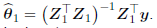 Thus, the principal component estimator of β in (2) is given by
 () 4
() 4
with covariance matrix 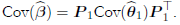
II. Simulation study
To evaluate the performance of the proposed principal-component-based method, we carried out a Monte Carlo simulation experiment with 20,000 replications on the stochastic frontier model
 () 5
() 5
with a half-normal/normal specification, 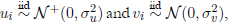 where σ
u = 3, σ
v = 2.5, σ
2 = σ
2
u + σ
2
v = 15.25, r = σ
2
u/σ
2 =0.59, (β
0, β
1, β
2) = (1, 0.8, 0.7); and (x
1, x
2) ~ N (µ, Σ) with µ = (20, 25) and
Σ
=
DRD
, where
D
= diag(σ
x1 , σ
x2 )= diag(1, 2); and
where σ
u = 3, σ
v = 2.5, σ
2 = σ
2
u + σ
2
v = 15.25, r = σ
2
u/σ
2 =0.59, (β
0, β
1, β
2) = (1, 0.8, 0.7); and (x
1, x
2) ~ N (µ, Σ) with µ = (20, 25) and
Σ
=
DRD
, where
D
= diag(σ
x1 , σ
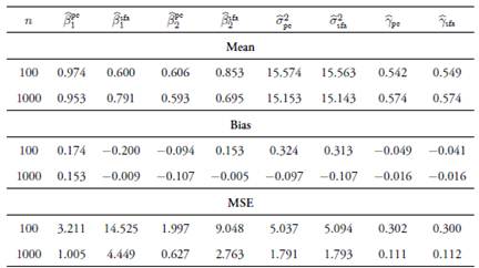
x2 )= diag(1, 2); and  with ρ = Corr(x1,x2) = 0.7, 0.8, 0.9. For the most severe multicollinearity prob lem, where ρ = 0.9, we performed the simulations with n = 1000 to study the large sample properties of the estimator. We used the frontier: Stochastic Frontier Analysis R package version 1.1-0 by Coelli and Henningsen (2013).
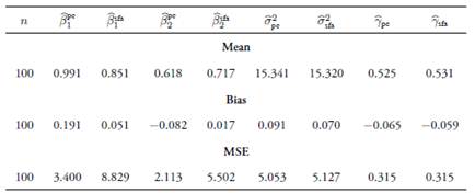
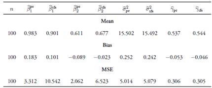
Tables 1-3 show the means, biases, and mean squared errors −MSE− of estimators of β
1 and β
2 approximated by the principal-component-based  and the usual stochastic frontier analysis
  methods for the assumed values of ρ. Results indicate that, in general, the coefficient estimators obtained with the principal-component-based method are biased, as these biases do not decrease asymptotically. However, the estimators have less MSE with respect to the ones obtained by the traditional method, even in large samples. The usual estimators are biased for finite samples with greater biases than for the proposed method, although these decrease asymptotically. The estimations for γ and σ
2 remain unaffected if the principal components are chosen correctly. Finally, when keeping fixed the number of principal components, the biases increase as the linear relationship among variables decreases.
methods for the assumed values of ρ. Results indicate that, in general, the coefficient estimators obtained with the principal-component-based method are biased, as these biases do not decrease asymptotically. However, the estimators have less MSE with respect to the ones obtained by the traditional method, even in large samples. The usual estimators are biased for finite samples with greater biases than for the proposed method, although these decrease asymptotically. The estimations for γ and σ
2 remain unaffected if the principal components are chosen correctly. Finally, when keeping fixed the number of principal components, the biases increase as the linear relationship among variables decreases.
III. Application
To see how the proposed solution behaves with real data, we use the production data of the agricultural and livestock sector with a sample of n = 23 livestock farms. The output variable is the total income, and inputs are labor, capital and other inputs; all have been measured in nominal Colombian −COL− pesos.
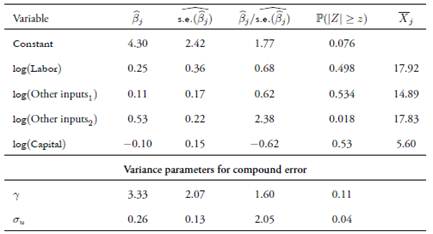
Then, a stochastic frontier production model was fitted assuming a Cobb-Douglas functional form with normal-exponential specification, 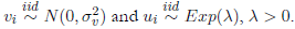 Estimations were carried out us ing the LIMited DEPendent −LIMDEP− econometric software (version 10). As can be seen in Table 4 the only statistically significant parameter is the input corresponding to log(Other inputs2). Although the variable log(Capital) is insignificant, its estimated coefficient has an unexpected opposite sign, indicating a signal of possible multicollinearity.
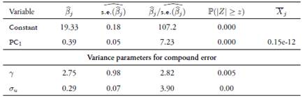
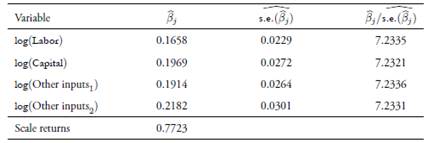
To detect multicollinearity, we computed the scaled condition in dexes. Table 5 shows there are two harmful condition indexes (with values greater than 30), indicating two possible near-linear dependencies among inputs. Thus, under the multicollinearity problem, we applied the proposed principal-component-based solution. The proportion of vari ance explained by the first principal component was 88.6%. Therefore, we applied the solution using this principal component. Table 6 displays the corresponding results. Based on these results, the estimates of the principal-component-based stochastic frontier using the equation (4) are in Table 7. Results show that all inputs are statistically significant with correct signs in accordance to production theory.
Conclusions
Based on simulation results, the estimators for inputs obtained under the proposed principal-component-based solution are biased, and such biases do not decrease asymptotically. Besides, the estimators have less MSE with respect to the usual ones even in large samples. For finite sam ples, the estimators are biased, and seem to have greater biases than the principal-component-based estimators. Also, the bias diminishes when the sample size increases. If the principal components are correct, the estimation of  remains are correct, the proposed method. Furthermore, when keeping fixed the number of prin cipal components, the biases of the proposed estimator increase as the linear relation between covariates decreases. The choice of the number of principal components is critical to the estimation of β, γ and σ2, as well as for the efficiency component. After applying the proposed method on real data from the agricultural and livestock sectors to evaluate its tech
nical inefficiency, our method seems to provide better estimation results for the coefficients, as well as for the scale returns, in comparison with the traditional method.

