




 Spanish (pdf)
 Article in xml format
 Article references

 Automatic translation
 Send this article by e-mail
 Cited by SciELO
 Cited by Google
 Similars in
SciELO
 Similars in Google

 Permalink


Introduction
The global energy demand increase and the well-founded hopes for reducing carbon emissions worldwide have led to significant interest in the scientific community in obtaining new ways of clean energy. Among the different renewable energy options, Marine energy represents a promising future that remains largely unexplored, considering that seawater covers more than 70% of the Earth’s surface 1 Because of its high utilization rate, power density, and predictability, wave energy is one of the most promising energy resources 2. An oscillating water column (OWC) could be a sustainable technology to generate electricity and it is considered a wave energy converter (WEC) 3. This energy can be used to diversify the energy basket and the distributed generation, satisfying the demand for electricity in the non-interconnected zones (NIZ) of Colombia 4. Given that in our country 15% of energy is expected to come from non-conventional sources of renewable energy (NCSRE) by 2030 5,6, and with the aim to contribute to a competitive, integral, diverse, safe and inclusive energy basket throughout the territory, especially in the NIZ, it is essential to advance towards the development, study and inclusion of new systems for the use of NCSRE. In the country, a mechanical system has been used to harness the energy of sea waves, where the lifting motion of a buoy where the elevation motion of a buoy is transformed into a rotational movement to generate energy 7. In turn, 8 investigated the selection of an oscillating WEC and power take-off (PTO) system for wave energy harvesting and determined that WECs coupled with to shore-based fixed structures and direct mechanical PTOs have significant advantages in terms of manufacturing, operation and service. In recent years, 9 made a review about the potential of hydrokinetic energy. In that work, the authors detailed that the use of renewable sources for energy production has been of great interest to the scientific community.
The effective use of Computational Fluid Dynamics (CFD) has allowed numerical simulations and analysis of OWC devices as an alternative to experiments. In this regard, the study of OWC operation can be conducted by using numerical models without incurring costly manufacturing tests. Taking into account what is described by López and coworkers 10, two groups of numerical models stand out for studying the behavior of OWC WEC: (i) the potential flow models that are solved under the Finite Element Method (FEM) and the Boundary Element Method (BEM), and (ii) the Reynolds-Averaged Navier Stokes equations (RANS). Particularly, RANS have the advantage of solving the velocity field in the whole domain and overcoming the limitations of nonlinearity, wave breaking, and dispersion, contrary to what several conventional wave models can do. OWC was first studied in the 1940s 11. For many years, great advances and studies have been made on these devices and they have even been built in countries such as Japan (1984) 12, Scotland (1985) 13,14, Portugal (1999) 3,15, United Kingdom and China (2001) 12,16, Ireland (2008) 13,16, Spain (2011) 12,16,17, Australia (2013) 13,18 and South Korea (2015) 3,16. Although this device has already been investigated in Colombia and other countries of the continent, from the authors’ knowledge, no major studies related to numerical modeling have been reported. Therefore, the main contribution of this work was to computationally simulate an OWC for the wave conditions of the coastal areas of Colombia, with low cost and environmental impact, simple in its manufacture, installation and maintenance, allowing the diversification of the energy mix and the distributed generation in NIZ and coastal areas of Colombia. Finally, in this research, the numerical simulation of an OWC adapted to the Pacific Ocean conditions at a laboratory scale was performed on the basis of CFD using the ANSYS-Fluent program running a numerical model for a 2D domain under the RANS equation solver with the Volume of Fluid (VOF) surface capture scheme.
Materials and methods
Fundamentals of an OWC
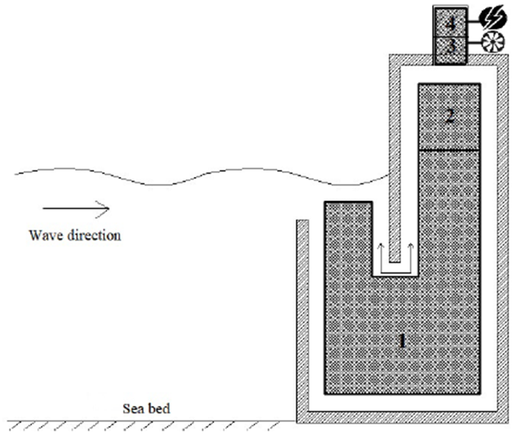
OWC is a simple column of water formed inside a chamber that is submerged partially in water, where an air column is readily formed in the enclosed region between the water column-free surface and the chamber ceiling and walls. The fall and rise of water depressurizes and pressurizes the air within the column, generating high-speed oscillatory currents through a small duct 19. Figure 1 illustrates the main components and regions over which an OWC can be divided. Region 1 corresponds to the U-shaped water column, Region 2 corresponds to the air column that is formed between the device chamber and the water surface. Regions 3 and 4 constitute the PTO system, which is the wave energy harvesting heart by restricting the air column movement. PTO enables pressure formation, inducing high-speed oscillatory air currents 19, and transforming pneumatic energy from ocean energy into electricity 3. Consequently, Region 3 corresponds to the zone where a Wells turbine is located, and Region 4 illustrates the zone where an electric generator can be located. On the other hand, a turbine, and a hollow pneumatic chamber are the main components of an OWC device 20. The former is coupled with an electric generator and the latter has a large opening below the water surface. In this device, both regular and irregular incident waves make the water column inside the resonance chamber to oscillate, forcing the air trapped above the water column to exit and enter the turbine periodically. The electrical generator is involved in the conversion of pneumatic energy into electrical energy. This kind of device can be adapted to several ocean conditions 20. Accordingly, two main stages are identified in the wave energy conversion process using an OWC. Initially for all, the wave energy is converted into pneumatic energy by the air chamber; and finally, this pneumatic energy is converted to electrical energy by a self-rectifying air turbine coupled to an electric generator through the PTO system 21 From the literature, the two energy conversion stages can be seen to be separated and individually investigated 22. That is the reason why this work presents the computational modeling of an OWC in its first stage, where the wave energy disturbs the air column periodically without considering the PTO system involving a self-rectifying turbine, the electrical generator and the cabling.
2.2 Wave resource
Wave characteristics
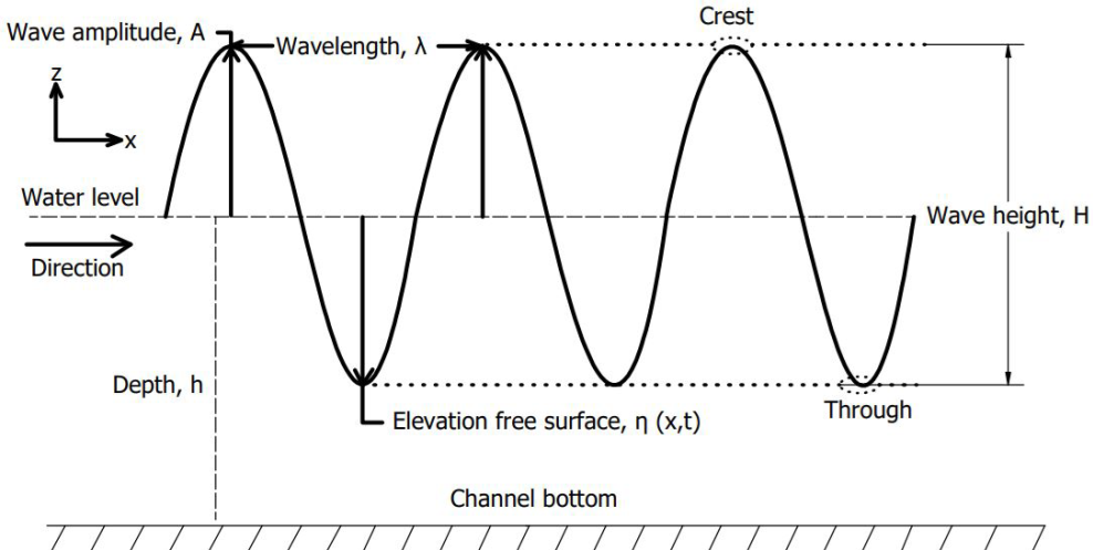
Several parameters characterize a wave. Among these parameters, the wave height (H), period (T), wavelength (λ) and amplitude (A) can be named, as well as the depth (h) and the free water surface elevation (η) over which waves are propagated, as illustrated in Figure 2. The free water surface elevation η(x,t) at any horizontal distance (x) and time instant (t) can be determined through Stokes second-order nonlinear theory [23] given by Equation (1).
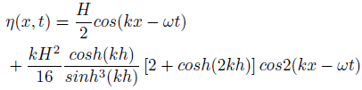
T can be calculated through Stokes theory given by Equation (2), k (wave number) and ω (angular frequency) can be calculated by 2π/λ and 2π/T, respectively. According to the values of λ=1.47 m and h=0.35 m; the analytical value of the period was 1.02 s. Therefore, during the investigation, values of k= 4.27 m −1 and ω= 6.15 rad/s were used.
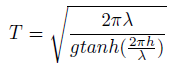
In this research, a scale factor (S) equal to 50 was selected to simulate the wave characteristics under a 1:50 ratio, as reported by 24-26 and coworkers. Taking into account: i) this S value (1:50) used to simulate in a wave channel the conditions of the Colombian Pacific Ocean, ii) T given by Equation (2), iii) the reduced scale wave length; it has been found that the incident wave energy content could be calculated as a function of h, T and H. In this paper, the study was performed for the wave conditions: H=0.02 m, λ=1.47 m and h=0.35 m, where the latter follows the conditions used by 27 in the wave channel.
Wave Theory
Figure 3 presents the validation limits of several wave theories, which were studied by Le Méhauté and coworkers 28,29.
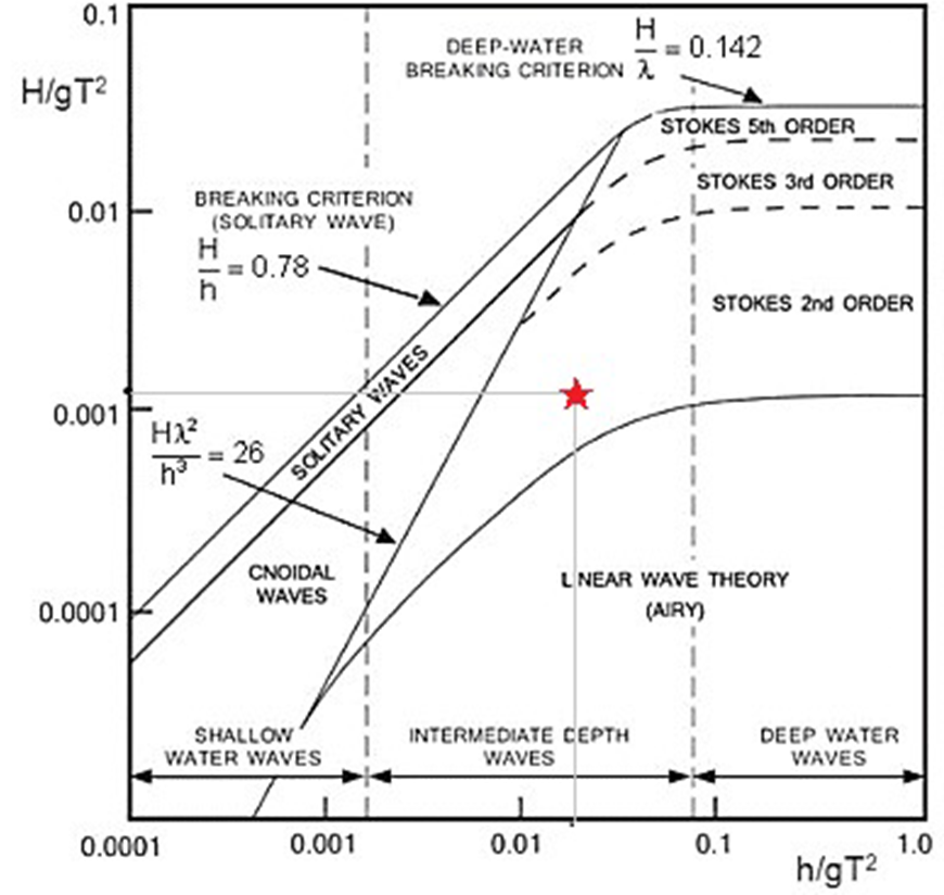
Figure 3 Le Méhauté diagram considering the Pacific Ocean wave conditions under different wave theories 29
In this research, considering the mentioned values (H=0.02 m, h=0.35 m, g= 9.81 m/s2 and T=1.02 s) and using the diagram provided by Le Méhauté shown in Figure 3, the most adequate wave theory was selected to analyze the wave conditions of the Colombian Pacific Ocean, the star shown in the figure indicates the theoretical region on which the numerical modeling was based. Consequently, Figure 3 shows that the linear theory for intermediate waters is adequate to represent the wave conditions.
Hydrodynamic parameters
The performance of an OWC (ε) can be evaluated by Equation (3) in terms of the ratio existing between the power of the incident wave (P inc ) and the pneumatic power obtained at the output (P out ), as defined by Alfonso et al.30.
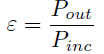
The power available during a wave period is given by Equation (4).

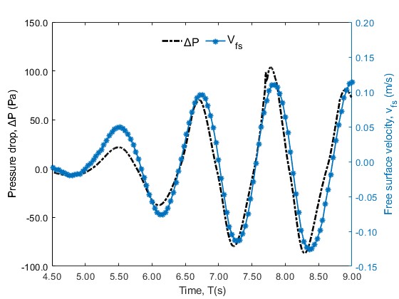
Following as described by Equation (4), the power available for the mentioned wave characteristics (H=0.02 m, λ=1.47 m and h=0.35 m) in a numerical wave tank (NWT) is 0.46 W/m. The average pneumatic power (P out ) for regular waves can be calculated by Equation (5), between an initial and final time period within the steady-state region of the measurements, where ΔP is the instantaneous pressure drop within the chamber, and Q(t) is the volumetric flux, which is defined for a 2D geometry as Q(t)= S chamber *V fs , where V fs is the free water surface velocity in the vertical direction (m/s) and S chamber is the area of the water plane of the OWC chamber, defined by b*w; where w is the OWC chamber width (in the dimension perpendicular to the wave propagation plane) which is assumed to be 1 for 2D computational modeling.

Where the free surface elevation in time at a given distance from the wave generator is denoted as η(x,t) and dt is the sample interval or step size used in the setup for ANSYS-Fluent.
Computational modeling
As for the computational modeling, the ANSYS-Fluent software was used to umerically solve the proposed case study adapted to the Pacific Ocean conditions, where the multiphase model using VOF was utilized for the two-phase water-air flow treatment.
Computational domain
Figure 4 shows the main dimensions and the boundary conditions of the NWT computational domain used within the ANSYS-Fluent interface. Five wave recorders (WG1-WG5) were placed throughout the computational domain to monitor the free water surface elevation. The separation between each wave recorder equaled the wavelength, WG5 was used to record the water elevation inside the resonance chamber. Two pressure monitors (SP1 and SP2) were placed at the top of the inner zone of the OWC air chamber to record the pressure drop, as reported by Wang et al.31.
Numerical simulation using CFD
The numerical simulation for the computational domain was performed under the laminar regime, unsteady state and incompressible flow, as used by 27,32,33 and coworkers. The VOF method has been used to correctly describe the interface between water and air 34-37; this model takes into account the interaction between these two fluids, where the volume of a phase is calculated through its volume fraction (α) 38. As indicated in 27, VOF considers a volume fraction (0 ≤ α ≤ 1) determining the fluid fraction in each elementary control volume in the domain. The equations of the amount of motion, continuity, and volume fraction were used to model the incompressible, laminar and unsteady flow of a mixture of water and air. As for the direct configuration in ANSYS-Fluent and for the advective terms treatment, the first-order upwind scheme was used. Additionally, the Pressure Stepping Option (PRESTO) was configured for the spatial discretization of the pressure in the momentum equation, and the couple scheme was used under the pressure-velocity coupling algorithm configured through the Pressure Implicit Split Operator (PISO) algorithm. During the simulation process, 0.001 s was the step time used with a maximum number of iterations of 35. In addition, the residual convergence criterion was set at 10 −6 (27. In this work, all the points of the free surface have an α of 0.5 28. The regular wave generation was performed at the left side channel boundary, which was named as inlet, where it was possible to generate a numerical wavefront by means of a Stokes wave generator directly from the program, using the open channel velocity input condition. To set the wavefront input directly from the software, wave H and λ values of 0.02 m and 1.47 m were used. For the pressure outflow conditions at the top of the channel and at the air outflow at OWC, a relative pressure of 0 Pa was used. The direction of the wavefront ranges from +X to -X. The no-slip condition was assigned to the channel bottom and the walls of the OWC, this condition has been widely used by authors such as 39-42 for the simulation of a wave channel and the walls of an OWC. It has been found that considering no slip allows capturing the boundary layer developed from the walls 11; generally, it is used at the bottom and side walls of the NWT, chamber and duct walls 42. This condition points out that the derivative of the volume fraction in time equals zero for the VOF equation 27. The simulation starts at t=0 s, at which time the fluids (water and air) were completely still. For the 2D analysis and as an indispensable part of a pneumatic type OWC device, the PTO system adopted here was modeled by using an orifice at the device top for the numerical simulations 31.
The domain used was initially modeled in Autodesk Inventor 2023 and imported as a surface within ANSYS Space Claim software.
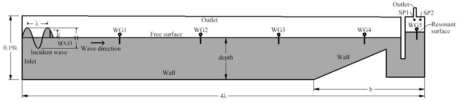
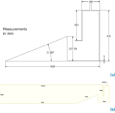
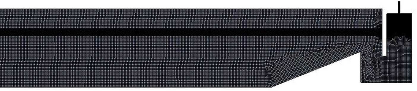
Figure 5 presents the geometry used. Figure 5a illustrates the dimensional details associated with the OWC used for the numerical simulation and Figure 5b presents the computational domain inserted as a surface in Space Claim. The mesh was generated using ANSYS-Fluent Mesh and refined mainly on the free water surface area, the channel walls and the OWC, places where a high level of detail and cell-to-cell information was needed for the simulation process. The mesh utilized in the numerical simulations is presented in Figure 6. CFD simulations were carried out using a LENOVO Thinkstation P520 Intel W2145 @ 3.7 GHz with 64 GB RAM, on each machine, using parallel processes. Each simulation took about 10 h.
Results and analysis
Initially, ensuring a good match between the mesh size and the time space for reliable CFD results was required. Consequently, a large number of simulations were conducted to determine the mesh quality influence in selecting the most appropriate mesh size in order to guarantee favorable results at low computational costs. For this reason, a structured mesh was performed in this research. On the other hand, it has been found that by comparing the simulations of the water-free surface with respect to the analytical models, accurate and reliable results can be guaranteed both in time and space 27,32,33. So to monitor η(x,t), a wave gauge (WG) was used. The first step during the simulation was to validate the wavefront for the Pacific Ocean conditions at a scale of 1:50 (λ=1.47 m and H=0.02 m). In Figure 7, both the numerical and analytical results obtained from the free water surface elevation through the wave recorder WG1, located at λ m from the wave generator were reported. The analytical results were obtained using Equation (1). Furthermore, to study the computational domain spatial independence, three meshes of different sizes were performed in this research. Since the fluctuations of the chamber-free surface are measured under the excitation of the incident waves 43, in this research, a wave height (H) of 0.02 m was used as a constant for all treatments.
Table 1 Mesh independence study
| Coarse | Medium | Fine | |
|---|---|---|---|
| Number of nodes Number of elements Max. skewness Max. aspect ratio Min. ort. quality | 75,371 74,074 0.994 30.907 0.067 | 159,535 157,551 0.996 30.103 0.069 | 349,554 346,680 0.846 38.575 0.246 |
Figure 8 shows the free water surface elevation curve around WG5 (in-chamber wavemeter) obtained from the simulations performed for a coarse, medium and a fine mesh. The comparison parameters, such as the mesh quality, number of nodes and the elements, are presented in Table 1. The mean mesh was used for subsequent simulations due to its good relation between the quality of the results and the computational costs. Moreover, the step size independence study was carried out to select the most appropriate time parameter. In this study, 0.001, 0.002 and 0.003 s were the step sizes studied whose elevation of the free water surface is presented in Figure 9. In order to have a good relationship between computational costs and the quality of the results, a step size equivalent to 0.001 s was chosen.
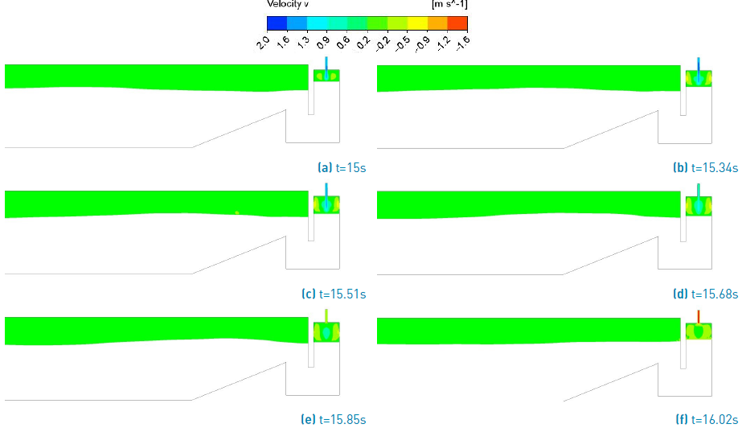
The water column motion generated by the incident wavefront adapted to the Pacific Ocean conditions can be characterized by the phase contour and the fluid velocity at progressive time instants. To this point, the wavefront took about 4.15 s to be reached from the wave generation zone to the resonance chamber. Figure 10 illustrates the phase contour for the NWT and the water column from 15 s to complete time period (T=1.02 s). During this time, the water surface variation inside the chamber can be appreciated. The red and blue colors represent water and air, respectively. Figure 11 represents the air velocity contour for the OWC studied during the process of ascent and descent of the water column. It can be seen that the air velocity was higher when leaving the chamber (V out = 1.97 m/s) than when entering the chamber (V in = -1.53 m/s). In this regard, 44 pointed out that the air velocity is not equal during the fluid inlet and outlet of the OWC. It has been found that the velocity is higher during the air outlet of the device chamber. This can be explained by the resistance effect from the water surface that is in the resonant chamber as air enters the device, resulting in lower inhalation velocities 45 Figure 12 illustrates the free surface vertical velocity and differential pressure within the resonance chamber for the simulation performed. As observed, the maximum pressure change was around 104 Pa under an absolute maximum V fs of 0.12 m/s. The maximum chamber efficiency and the mean free surface velocity inside the chamber was 67.2% and 0.12 m/s, respectively. Therefore, optimizing the chamber shape parameter for the wave characteristics is required to improve its operational efficiency. At present, the country lacks the development of these devices, but there are high hopes that wave energy could represent one of our most important energy sources in the coming years in a clean and affordable way. Rezanejad et al.46 found efficiencies of up to 59.1% for a T and a wave H of 1.05 s and 0.02 m, respectively: This result is very close to the one achieved in this research under regular waves. However, the referred authors did not consider in their OWC the inclined ramp and U-shape that Vyzikas et al.47 did use in their research and that were considered in this paper. In turn, Shahabi and collaborators 37 found a maximum efficiency of up to 67% for a geometry that sets the basis for the shape of the chamber studied in this work; nevertheless, the study was through a constructive design, observing the sensitivity of the geometric factors simultaneously. In contrast, here, the computational model was performed for a single geometry, such as the one presented in Figure 4.
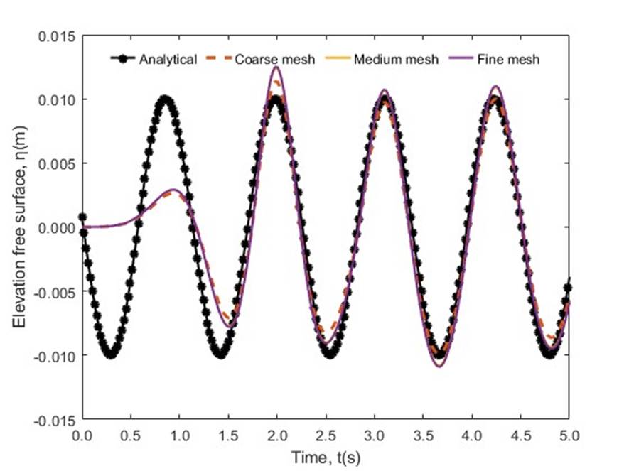
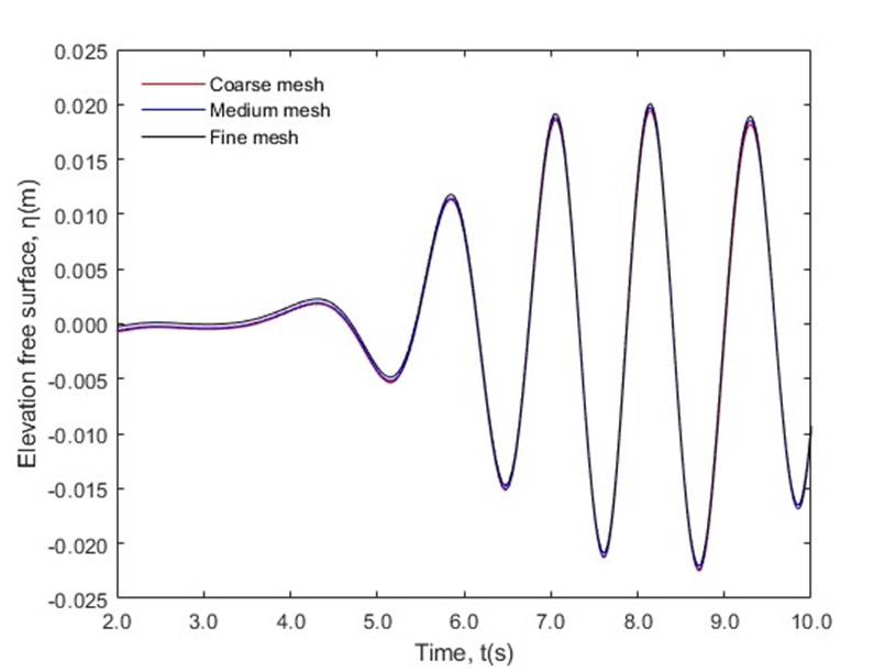
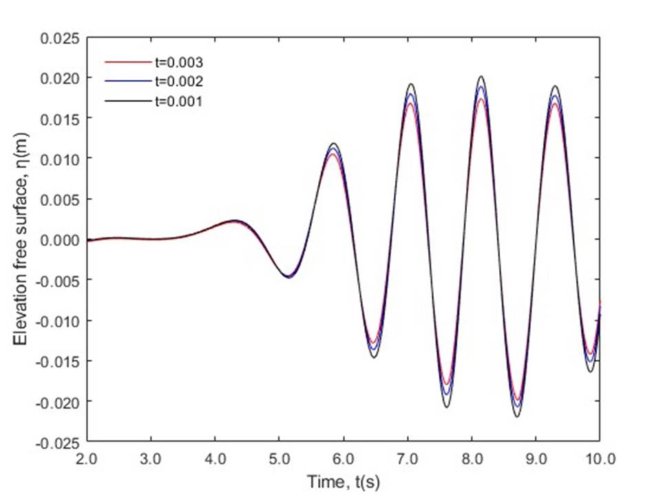
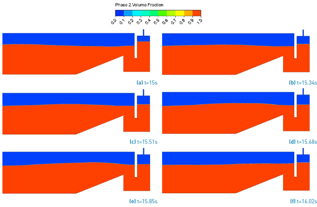
Figure 10 Phase contour at successive time instants for computational model where red color indicates water and blue color indicates air
Conclusions
In this research, it was possible to numerically simulate the OWC hydrodynamic behavior adapted to the conditions of the Colombian Pacific Ocean at laboratory scale using ANSYS-Fluent, RANS and VOF to deal with fluid motion and free water surface. The maximum efficiency obtained from the chamber was 67.2% and the average velocity of the free surface of the water column for the geometry studied was 0.12 m/s. In this regard, the OWC can be a sustainable technology to generate electricity in Colombia using the resource available in the Pacific Ocean.

