1 Introduction

Identification problems in some basic differential equations play an important role in many branches of science and engineering. Several discretizations are reported to numerically solve the elliptic problem. However, when it comes to solving an inverse problem such as finding a coefficient, numerical approximation schemes can give undesired results and even more so when the information presented is contaminated with noise. The discretization of the problem is done using two difference quotients which is a regularization strategy (see [¹]) can solve the problem and molification smooth the desired result. Hinestroza and Murio introduced a modification method for the identification of coefficients (see [²]). In this paper we consider the inverse problem of identifying the coefficient: find the thermal conductivity a(x) > 0 in the parabolic equation:

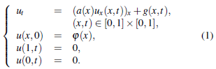
in the (1) equation, g(x, t) and u(x, t) and φ(x) are given or partly known, the subscript x denotes derivative with respect to the variable x. In addition, α(x) > 0.

By these conditions, we will denote

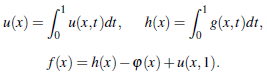
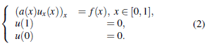
Then, we reduce (1) to the elliptic equation as a inverse steady heat conduction problem (2).

If ux does not vanish anywhere in (2) and α(0) = 0, we can identify a explicitly as

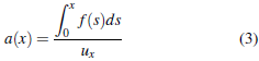
Therefore, it is determined uniquely. So, in order to calculate a, one has to differentiate u, which is an Ill-posed problem (see [¹]).

Furthermore, there is another effect of instability from the division by u _x in (3): in regions where u _x is small, errors, for example, f can occur, which is not surprising since when u _x vanishes, α cannot be determined at all, so some instability must be expected where u _x is small. This is a nonlinear effect, while pool conditions involved with differentiation data derived from the fact that the linearized problem is too bad. We emphasize that, in general, the parameter identification is a nonlinear inverse problem, even if the underlying equation is (for a known parameter) a linear equation. This, coupled with inverse problems in heat conduction and inverse scattering problem (see [³]), are strong motivations for the study of nonlinear inverse problems.

This paper is organized as follows: In section 2 we present the Two different quotients method. In section 3 we will show the modification method for the identification of coefficients that would allow smoothing the estimate of the coefficient and show examples of parameter estimation under conventional discretization methods and will be compared with the double quotient discretization method. Then, the estimate will be smoothed by mollification method.

2 The two different quotients discretization method

To reconstruct α in (2), we take into account temperature measurements.

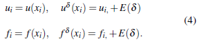
where i = 1, ・ ・ ・ ,n and E(δ) is noise, which depends of δ.

Then, we reduce (1) to the elliptic equation as a inverse steady heat

The discretization of the problem is done (2) using two difference quotients which is a regularization strategy (R _h y) (x) (see [¹]).

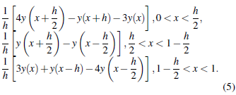
Where regularization parameter α = h is the step size in (5). Having the problem written in this form

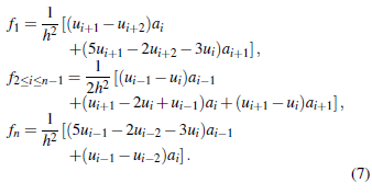
Where A(u) is non singular. The discretization equation (2) can be taken to the form fi for i = 1 , ∙∙∙, n by equation (7).

3.1 Noise generation for the system A(u)α = f

For the Aα = f matrix system obtained under discretization methods (7) that follows approximate the estimate of the fractional a(x) > 0 we introduce a noise of the order of 10^-2:

where E is a noise vector whose entries are chosen from a normal distribution with mean 0 and variance 1, so that:

3.2 Smooth by mollification

We use the Gaussian Kernel ψ _h by

and the convolution

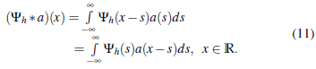
For more information on the mollification method see [¹].

3.3 Numerical examples

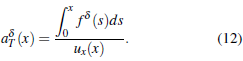
In the following examples, f(x), u(x) and a(x) are given to satisfy problem (2). Therefore, we will denote the exact solution as α, a ^δ _T is the approximation of α by using trapezoidal-rule quadrature with n - 1 trapezoids that approximate the integral given in equation (3) whose integrand is perturbed as shown in equation (8) to obtain the following equation:

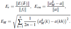
Given n = 64 data that defines the problem, calculate the step size h = 1/(n - 1). We denote by α ^δ _R the solution of system A( u) α ^δ _R = f ^δ which originates through the discretization of equation (7). Finally, we denote by α ^δ _m the smoothing of the approximation solution α ^δ _R by Mollification, see section 3.2. We also note by E _r as the relative error of approximating f with f ^d , E _rm as the relative error of approximating a with α ^δ _M and the error E _M as error by molification defined as:

exmp 1 Consider the functions f,u and a given in the numerical example 1 of ([ ⁵]).

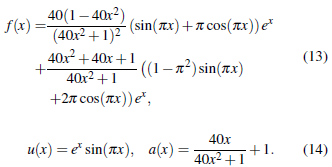
Figure 1shows the graphs of f and f ^δ , where it can be seen that the induced noise is less than 0.01 (E _r = 0.01), zooming allows you to see the difference between the two functions.

Figure 1: Numerical f and f ^δ . Example 1. 

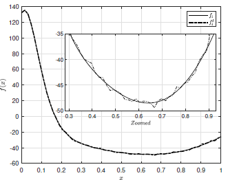
Figure 2shows Exact Solution a which is continuous for all x Є [0,1] and numerical solution without regularizing under the trapezoidal method α ^δ _T that presents an asymptotic behavior αt x = 0.598 when u _x vanishes, see equation (12).

Additionally, its approximation in its entire domain is not good and for some values ofx, the function a(x) < 0.

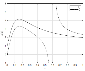
Figure 2: Exact Solution a and numerical solution without regularizing under the trapezoidal method α ^δ _T . Example 1. 

Figure 3shows that the discretization of equation (7) regularizes the problem and allows a good approximation of a, note that the approximation does not have an asymptotic behavior.

Figure 3: Exact Solution and numerical regularized solution α ^δ _R . Example 1. 

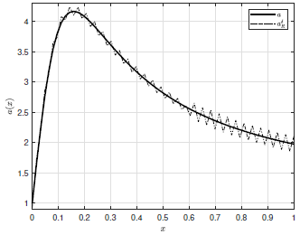
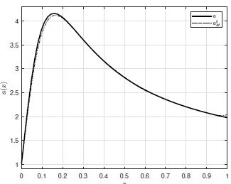
Figure 4shows α ^δ _M , the smoothing of the approximation solution α ^δ _R by Mollification. where it is observed that the solution α ^δ _R shown in Figure 3 is smoothed, and a good approximation to the exact solution is obtained as indicated by the respective errors E _rm = 0.0124 and E _M = 0.12825.

Figure 4: Exact Solution and numerical regularized solution α^δ _R by Mollification. Example 1. 

exmp 2 Consider the functions f,u and a given in the numerical example 1 of ([ ⁴]).

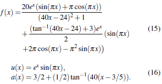
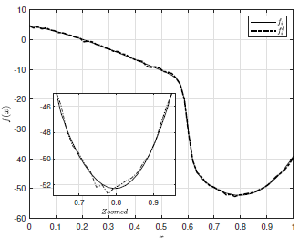
Figure 5shows graphs of f and f ^δ , in this example E _r = 0.0097.

Figure 5: Numerical f and f ^δ . Example 2. 

InFigure 6you can see again the asymptotic behavior where by trapezoidal method make that for some values of x the function a is negative. It can also be seen that the regularization method allowed us to approximate the functional α.

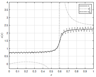
Figure 6: Exact Solution, a and numerical solution without regularizing under the trapezoidal method α ^δ _T and numerical regularized solution α ^δ _R . Example 2. 

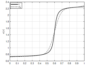
Finally, inFigure 7it is smoothed by mollification to the regularized solution and the errors E _rm = 0.0419 and E _M = 0. 0583 were obtained.

Figure 7: Exact Solution and numerical regularized solution α ^δ _R by Mollification. Example 2. 

4 Conclusions

The derivative regularization method proposed by Kirch applied to self-adjoint elliptic equations to solve the ill posed inverse problem of finding the conductivity coefficient; it is easy to program and shows very good results compared to the proposed methods and examples. In the examples, mollification was used to smooth the graphs and not as a regularization method. [⁴, ⁵]. It would be interesting for the future, a comparison with other methods or at least show the complexity of the proposed method compared to traditional ones. Although due to space limitations it would be interesting to see the convergence.