1 Introduction

Classification algorithms can be roughly categorized into dissimilarity-based classifiers, probabilistic classifiers and geometric classifiers [¹]. The first ones assign an unlabeled object -represented as a feature vector x - to the class of the most similar examples within a set of either labeled feature vectors (also known as training objects) or within models previously built from them; the second ones estimate class-conditional probability densities by using the training objects and, afterwards, assign class labels to the un- labeled ones according to the maximum posterior probabilities; the third category of classifiers directly construct boundaries between class regions in the feature space by optimizing criteria such as classification error and maximum margin of separation between classes. The Nearest Neighbor (1- NN) rule is the paradigmatic example of the dissimilarity-based classifiers; it is very natural, intuitive for non-experts [²] and exhibits a competitive classification performance provided that a large enough training set is available. Several variants have been proposed to improve 1-NN, among them the so-called Nearest Feature Line (NFL) classifier [³] that enlarges the representational power of a training set of limited cardinality by building a linear model (a feature line) between each pair of training feature vectors of the same class.

Even though NFL effectively counteracts the weakness of 1-NN under representational limitations, it is much more costly than 1-NN and also introduces two drawbacks: interpolation and extrapolation inaccuracies (see Section 2.1.1) that are reflected into high classification errors in problems having particular data distributions and dimensionalities. Both drawbacks of NFL were diagnosed in [⁴], whose authors also proposed the so-called Rectified Nearest Feature Line Segment (RNFLS) classifier as a solution to the inaccuracies of NFL via two processes called segmentation and rectification of the feature lines. Unfortunately, such an improvement of NFL is paid with a significantly increased computational cost for RNFLS, turning its application too time demanding. In spite that most of the computations in RNFLS are associated to the rectification process -which is only performed during the training stage and, therefore, off-line-, current application scenarios often imply the classification of evolving streaming data[⁵] that, after detecting changes in their distributions, demand an automatic retraining of the classifiers in order to quickly adapt them to new data behaviors.

An additional and often ignored motivation for speeding up classification algorithms is enabling the practitioner to perform fast simulations, in such a way that varying parameters and exploring different configurations over several runs of the classifier become feasible in reasonable amounts of time. Such simulations typically require the repeated estimation of the classification performance. Among the classical performance estimation methods [⁶], the so-called leave-one-out method is very often preferred be- cause it does not imply random splits of the data into training set and test set and, therefore, reported performances can be exactly confirmed by other researches; in addition, leave-one-out is approximately unbiased for the true classification performance [⁷][p. 590]. However, these desirable properties are obtained at the expense of a significant computational effort since the classifier must be trained as many times as the number of objects in the data set.

In recent years, the above-mentioned computational challenges have motivated an increasing interest in developing efficient implementations for classification algorithms, particularly those that are aimed to exploit technologies currently available in personal modern computers such as multi- core processors (multi-core CPU) and general-purpose graphics processing units (GP-GPU). Parallel implementations on the first ones are of special interest because, nowadays, they are omnipresent in domestic machines. Even though the second ones have become very popular, they are still not considered part of the default specifications for commercial computer ma- chines. A throughout study on GPU-based parallel versions of several ma- chine learning algorithms is carried out in [⁸], including implementations for well-known classifiers such as neural networks and support vector machines. In contrast, classifier implementations for multi-core CPU are scattered in the literature; for example the following, just to cite recent ones per each classifier category: A dissimilarity-based classifier - parallel implementation of the k nearest neighbor rule [⁹] tested on machines having from 2 up to 60 processing cores; A probabilistic classifier - the implementation in [¹⁰] of the naïve Bayes classifier, whose authors evaluated their algorithm on the publicly available KDD CUP 99 dataset; A geometric classifier - the so-called scaling version developed in [¹¹] for support vector machines, that was exhaustively studied for several threads/cores ratios. Nonetheless, to the best of our knowledge, neither NFL nor RNFLS have been studied for parallel implementations except for our own preliminary attempts: [¹²]. Therefore, in this paper, we propose parallel CPU-based versions for the leave-one-out test of both NFL and RNFLS by accordingly reformulating their tests in terms of a number of available computing cores and giving a thorough experimental evaluation of the proposed parallel evaluations.

The remaining part of this paper is organized as follows. The serial algorithms of NFL and RNFLS are presented in Sec 2.1. The proposed parallel implementations of the leave-one-out test for NFL and RNFLS are explained in Sec. 2.2. In Sec. 3, we present experimental results of the execution of the multi-core versions on several benchmarking data sets and compare them to the execution of their serial counterparts. Finally, our concluding remarks are given in Sec. 4.

2 Methods

2.1 Serial Algorithms

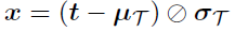
Let T = {( t ₁ , θ ₁), . . . , ( t _N , θ _N )} be the training set, with training feature vectors t _i ( RK and class labels θ _{i ( (} ω ₁ , . . . , ω _{C (}. Since feature values may have different dynamic ranges, it is customary to normalize each t _i by the mean feature vector ( µ _T ) and the vector of standard deviations per feature ( σ _T ), as follows:

where ø denotes the Hadamard (entrywise) division; notice that, in case that any entry of σ _T is 0, it must be replaced by 1 in order to avoid a division by zero. The normalized training set is thereby X = {( x ₁ , θ ₁), . . . , ( x _N , θ _N ) . Similarly, given a test feature vector t (RK , its normalized version x is obtained by

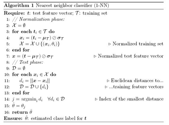
1-NN Classifies x according to the class label of its nearest neighbor in X. In more formal terms, the class label θˆ that 1-NN estimates for x is given by

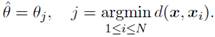
A detailed pseudocode for 1-NN classification is shown in Algorithm 1.

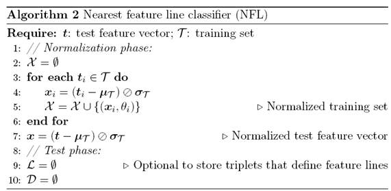
2.1.1 Nearest feature line classifter (NFL) One of the disadvantages of 1-NN, pointed in [¹³], is that 1-NN losses accuracy when |T | is small. In order to enrich the representational power of T , Li and Lu [³] proposed NFL that builds a set -denoted hereafter by L- of feature lines, each one connecting a pair of training feature vectors that belong to the same class. Since a line is geometrically specified by the pair of points it connects, each labeled line L _i can be represented as the triplet ( x _j , x _k , ρ _i ), where ρ _i is the class label of the feature line. Clearly, ρ _i is equal to both θ _j and θ _k since feature lines are restricted to connect class-mates.

NFL classifies x according to the class label of its nearest feature line in L; that is,

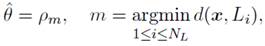
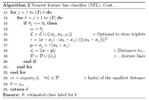
where N _L is the number of feature lines. A detailed pseudocode for NFL classification is shown in Algorithm 2.

2.1.2 Rectifted nearest feature line segment (RNFLS) classifter NFL suffers from two drawbacks: interpolation and extrapolation inaccuracies. Du and Chen [⁴] diagnosed both problems and proposed a modified version of the classifier, called rectified nearest feature line segment (RN- FLS), that includes two additional processes to overcome the inaccuracies: segmentation and rectification. The first one consists in computing the dis- tance from x to the feature line exactly as done in the NFL algorithm only if the orthogonal projection of x onto the feature line lies on the interpolating part of the line; otherwise, the distance is replaced by the distance from x to either x _j or x _k according to the side of the extrapolating parts of the line where the orthogonal projection of x would appears.

The second process -rectification- consists in checking whether the feature lines violates the territory of other classes or not; in case of violation, that line is excluded from and, thereby, it is not taken into account to compute the distances. A feature line violates the territory of other classes if there exists at least one training object for which the radius of its territory is less than its distance to the feature line. For each training object, the radius of its territory is defined as the distance to the closest training object belonging to a different class. A detailed pseudocode for RNFLS classification is shown in Algorithm 3.

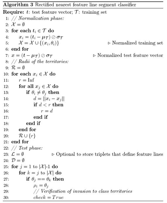
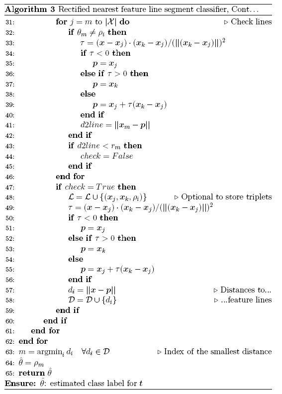
Notice that, in Algorithm 3, the second inner loop starts with k = j instead of k = j + 1 as in Algorithm 2. This difference is because RNFLS is defined to also include degenerated feature lines; that is, those lines connecting points with themselves.

2.2 Proposed parallel algorithms

The parallel programs for the leave-one-out evaluation were implemented in two phases: Preprocessing (P) and Classification (C). Figure 1 shows the preprocessing and classification steps, the sequence of functions, their associated complexity and which ones are running in parallel or in sequential mode. Each step is described in Sections 2.2.1 and 2.2.2.

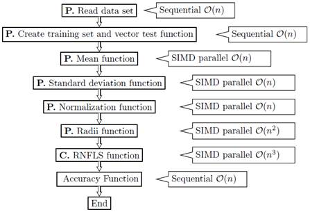
Figure 1: Block diagram of RNFLS algorithm. Mean, Standard Deviation and Radii functions are written in parallel using Single Instruction Multiple Data (SIMD), in front of each one their complexities are shown. 

The first step is loading the data set, then a storage structure (shown in Figure 2] is created by the Create training set and vector test function, this structure contains: (i) the training set T(i) and the test vector t ⁽ⁱ⁾ where 0 < i < N and N stands for the number of partitions; (ii) the mean feature vector µ _T = 0; (iii) the standard deviations vector per feature σ _T = 0 for both NFL and RNFLS are initialized in zero and also the algorithm calculates the radii vector R(i) = 0 initialized in zero too, only for the RNFLS algorithm. After that, the mean parallel and the standard deviation functions are calculated for each T(i) (see Figure 2]. These two vectors are used in order to normalize each T(i) and each t ⁽ⁱ⁾ , resulting X ⁽ⁱ⁾and x ⁽ⁱ⁾ , see Figure 3. So, each thread executes the NFL and RNFLS algorithms over each position of the structure in an independent way as shown in Figure 2. The size of the structure depends on the number of rows containing the initial data file.

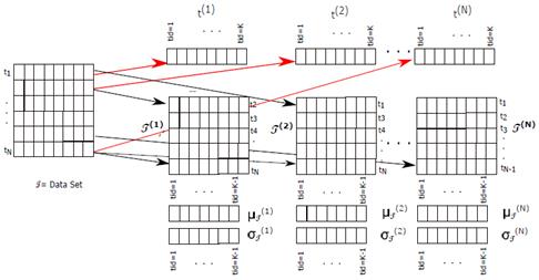
Figure 2 Leave-one-out parallel representation for RNFLS, mean µ and standard deviation σ parallel representation. 

2.2.1 Preprocessing phase In this phase, we use the SIMD Flynn taxonomy to implement parallel functions for computation of standard deviation, mean, radii, training matrix and test vector normalization (see Figure 1]. This section describes the algorithms involved in the preprocessing phase.

Figure 3: Structure after normalization for threads executions. 

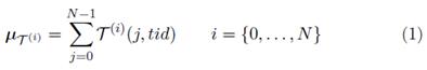
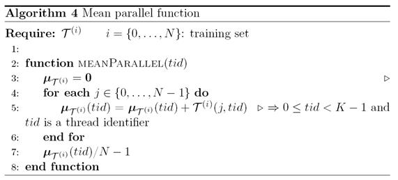
Mean parallel function (Algorithm 4) To parallelize the average of each training set X(i), as many threads are created as columns in the training set, each thread is identified with its tid where 0 tid < K-1 (K is the number of columns), so tid is used as a column index for the training set T(i)(j, tid). Each thread stores the results of the executions of the mean function in a temporal vector called µ _T (i) , where each vector position is calculated for a thread through their respective tid, leaving the result of executing the mean function in the same tid vector position, each thread obtains the average of each T(i)(j, tid) column, in a independent way, see Figure 2. The mean parallel function is shown in Equation (1). The mean function complexity for each thread is O(n).

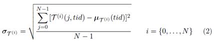
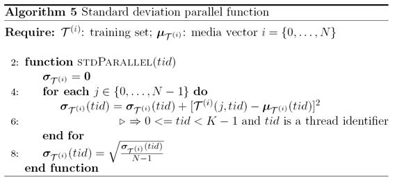
Standard deviation parallel function (Algorithm 5) The paralelization of the standard deviation σ _T is similar to the media parallel function method, as many threads are created as columns in the training set, each thread is identified with its own tid where 0 tid < K-1, the tid is used as index for the T(i) training set columns, each thread stores the standard deviation function results in a temporal vector called σ _T (i) , each position of σ _T (i) is accessed by a thread through their respective tid, leaving the standard deviation function results in the same tid vector position, each thread executes the standard deviation for each T(i)(j, tid) columns in an independent way (see Figure 2]. This function has the same complexity that Algorithm 4. The standard deviation parallel function is shown in Equation (2).

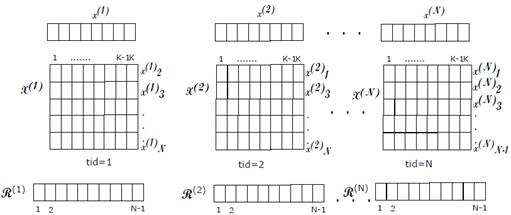
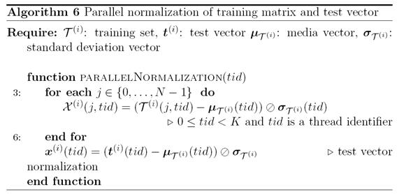
Training matrix and test vector normalization parallel function (Algorithm 6) Similarly, we apply σ _T (i) and µ _T (i) to its corresponding T(i) in order to normalize the training set and obtain X(i) as a result (see Figure 3). The process is represented in Equation

(3). It is important to note that we use the same structure T(i) in the program to store the normalized results. Each thread obtains the value of µ T (i) (tid) and σ T (i) (tid) in order to normalize each column element in T (i)(j, tid).

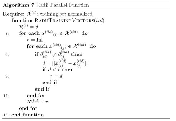
Radii parallel function (Algorithm 7) The radii function computes the territories of the each object in the data set. This function creates the radii vector for each X(i) implementing the segmentation into blocks of the “Radii of the territories” part in the RNFLS algorithm described in Algorithm 3. The parallel process redistributes on the cores of the machine the structure created in Figure 2; each core calculates the complete radii function code. Algorithm 7 shows how the structure distribution is performed.

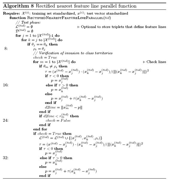
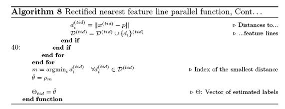
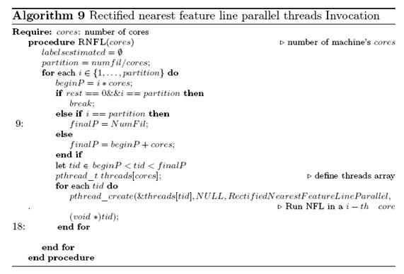
2.2.2 Classification phase The classification phase implements the NFL and the RNFLS algorithms, redistributing in each case the function over the machine cores and processing data that are on the positions of the structure according to the identifier of each thread. Algorithm 9 shows how the function is loaded using initial and final range partitions, according to the number of cores. For example, if the machine has 48 cores, each time the machine sends 48 processes to process the data in the structure shown in Figure 3. Each thread calls Algorithm 8, which verifies the invasion to class territories and calculates the best distance to each test vector x ^(tid) with respect to X (tid) and leaves the result in a vector Θ _tid of estimated labels in the corresponding tid position, making in parallel each leave-one-out test.

3 Results and discussion

The experiments were run on a Dell server with two (2) Intel(R) Xeon(R) CPU E7−4860 v2 @ 2.60GHz, each one with 12 real cores (24 cores in total and 48 Hyper−Threading), operative system GNU/Linux, Scientific Linux 3.10 for x86_64, using postfix threads, C library and Hyper−Threading (HT). The following data sets, taken from the UCI Machine Learning Repository (https://archive.ics.uci.edu/ml/datasets.html), were em- ployed for the experiments: Iris, Wine, Glass, Ionosphere, Bupa, WDBC and Pima.

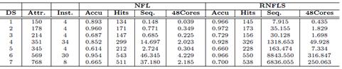
Algorithms 2 and 3 were run 20 times each one. Results shown in Table 1 are the mean of the executions for the sequential and the most parallelized versions; that is, using one core and 48 cores, respectively. These results illustrate how efficient an algorithm turns out if it can be adapted to a multi-core architecture.

Figure 4 shows that an acceptable performance of the algorithm is reached at around 24 cores, presenting a similar behavior when we increase the number of cores to 24, . . . , 48. Such a behavior is due to the Amdahl’s law limitation and other aspects such as low-level kernel primitives, shared memory and how the machine scheduler attends the threads¹.

Figure 4 (left) shows the elapsed times achieved for the smaller data set called, iris with 150 samples and 4 attributes and Figure 4 shows the elapsed times achieved for the largest (right) data set called WDBC with 569 samples and 30 attributes running the leave-one-out test with the NFL algorithm. For sequential versions of iris, the time was 0.148 sec and the parallel time with 48 cores was the best time 0.038 sec, with an speed up of 3.79 times best than the sequential version. For the sequential version of WDBC the time was 46.35 sec and the parallel time with 48 cores was the best time (4.23 sec), with an speed up of 10.96 times better than the sequential version. A similar behavior happens with the RNFLS version, see Table 1.

Table 1: Sequential and parallel Elapsed time (in seconds) of the small and bigger data. 

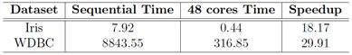
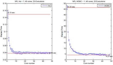
Figure 4: Elapsed time for the smallest data set (on the left) and the largest data set running Leave-one-out with NFL. 

In each run, we were careful in throwing one thread per core without surpassing the total Hyper-Threading that the machine can support in order to avoid overload and context change of the threads by the scheduler, in this architecture we can use 2 threads by core. When the number of threads exceeds 24 cores, the behavior of the speed-up changes, presenting ups and downs around 24 cores; see Figure 5. We note that the efficiency is achieve when each algorithm uses only the real base core equivalents (BCE) [¹⁴]. In spite of that, when we use the total capacity of multi- threads, the parallel algorithms (NFL and (RNFLS), achieve efficiency but not as significant as with the BCE.

Figure 6 and Figure 7 show the elapsed time and speed up achieved with the leave-one-out test using the NFL and RNFLS algorithms. The speed up was calculated with an approximation of the Amdahl’s formula S _up = Et _s /Et _p [¹⁵], where Et _s is the elapsed time of the sequential version and Et _p is the elapsed time of the parallel version using from 2 to 48 cores. Table 2 shows results for all the data sets used in these tests.

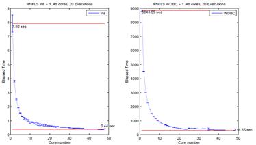
Figure 5: Elapsed time for the smallest data set (on the left) and the largest data set running Leave-one-out with RNFLS. 

Figure 6: Average speed up for all data sets running the leave-one-out test with the NFL algorithm. 

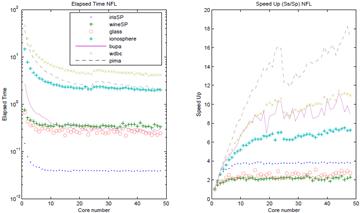
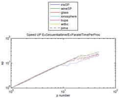
Figure 7: Average speed up for all data sets running the leave-one-out test with the RNFLS algorithm. 

Table 2: Elapsed times in seconds (parallel vs. sequential), for the leave-one-out evaluation of NFL and RNFLS using ANSI C. Data sets (DS): (1)Iris, (2)Wine, (3)Glass, (4)Ionosphere, (5)Bupa, (6)WDBC, (7)Pima  

4 Conclusions

The leave-one-out test was parallelized and tested with the NFL and RN- FLS algorithms, observing that the best acceleration is achieved under the actual machine base architecture (24 cores) and that multi-threaded activations, although they improve performance, do not achieve accelerations that exceed those achieved when using the base cores of the machine; the latter demonstrates that the acceleration of the algorithms is controlled by the limit imposed by the Amdahl’s law. The tests of the algorithms were repeated 20 times for each dataset in order to demonstrate the stability of the implementation, obtaining results with low standard deviations with respect to the mean. By using more threads than real machine cores, the clock speed of the cores decreases, this is a typical behavior of the Xeon processors to keep the heat levels generated by the processors stable when they are working at 100% of their capacity, which also affects the accelera- tion of the algorithms. It is important to note that the parallel functions for average, standard deviation and normalization do not behave efficiently for small datasets. The results showed that, using algorithms based on multi-thread multi-core architectures, an improvement of the leave-one-out test can be achieved with the RNFLS algorithm of 29.91 times compared against the sequential algorithm