Serviços Personalizados
Journal
Artigo
Indicadores
-
 Citado por SciELO
 -
 Acessos
Links relacionados
-
 Citado por Google
 -
 Similares em
SciELO
 -
 Similares em Google
Compartilhar
DYNA
versão impressa ISSN 0012-7353versão On-line ISSN 2346-2183
Dyna rev.fac.nac.minas v.78 n.168 Medellín out./dez. 2011
MOTION DETECTION ON FIXED CAMERAS SUBJECT TO VIBRATION
DETECCIÓN DE MOVIMIENTO EN FIJAS CÁMARAS SUJETAS A VIBRACION
HUGO JIMENEZ-HERNANDEZ
Centro de Ingeniería y Desarrollo Industrial. hugojh@gmail.com
JOAQUIN SALAS
Centro de Investigación en Ciencia Aplicada y Tecnología Aplicada. Instituto Politécnico Nacional. jsalasr@ipn.mx
Received for review October 7th, 2009; accepted August 10th, 2010; final version August, 20th, 2010
ABSTRACT: This article presents a new method for detecting moving objects in fixed cameras that undergo unexpected motion due to vibration. In our approach, the vibration is automatically compensated for using a dynamically-selected set of trackable features, computing frame-to-frame homographies while preventing numerical degeneracy. One of the most noteworthy characteristics of our method is its ability to withstand occlusions. The robustness of the method is demonstrated in situations where a monitoring camera is subject to vibrations due to inclement weather conditions, such as rain or wind, or other outdoor operating conditions, including vehicles passing nearby.
KEYWORDS: Dynamic selection of features, vibrations, motion detection
RESUMEN: Este trabajo se presenta un nuevo método para detectar a los objetos en movimiento cuando la cámara es afectada por vibraciones. En la propuesta, las vibraciones son compensadas mediante una selección dinámica de características seguibles. Dichas características son utilizadas para estimar una transformación homográfica entre cada par consecutivo de imágenes, mientras que no exista degeneración numérica en el sistema. Una de las mayores contribuciones del método propuesto consiste en el manejo de oclusiones. La eficiencia del método es probado en escenarios donde la cámara está afectada vibraciones causadas por las condiciones climáticas (como lluvia o viento) o por las exteriores condiciones de operación (como el paso de vehículos cercanos a la cámara).
PALABRAS CLAVE: Selección dinámica de características, vibraciones, detección de movimiento
1. INTRODUCTION
Most automatic image analysis algorithms in surveillance and monitoring applications operate under the assumption that the cameras remain fixed. However, this is difficult to enforce in realistic long-term applications where environmental conditions such as gusty winds, rain, or passing vehicles challenge this assumption. These vibrations cause the visual impression that everything is moving in the camera's field of view. The objective of this research is to provide a method for distinguishing between static and non-static objects in scenarios observed with cameras subject to the effects of vibrations. In [24], Tomasi introduced a method for extracting the tridimensional structure of a scene from a set of prominent features. These features were the result of the analysis of the structural tensor done by Shi and Tomasi [19] and a tracking method first introduced by Lucas and Kanade [21]. Recently, other scale-invariant descriptors have been developed by Lowe [18]. Based on this concept of saliency, we introduce a method for removing the effects of vibration from a set of trackable features, even when some of these features may be occasionally or permanently occluded, or their geometrical properties may be evolving as the image stream progresses.
The dynamic use of features leverages certain algorithms, specifically those depending on scene references, in order to improve robustness for a wide spectrum of changes. Consider, for instance, the use of features in tasks such as the characterization of moving objects [8], image registration using a particle filter [6], characterization of the objects' topology [23], optical flow [19], segmentation [16], and tracking [4,12]. Overall, these methods illustrate how the dynamic selection of features empowers algorithms to obtain better descriptors. Nevertheless, they assume vibration-free scenarios in which the camera remains fixed.
There are several methods to register images based on the dynamic selection of features. One of the most widespread is the random sample consensus (RANSAC) [11]. Recently, Lacey et al. [17], and Chum and Matas [7], introduced the sequential probability ratio test (SPRT) [26] into the RANSAC framework. Their method seems to perform better when the scenario contains only static objects.
In this paper, we present an algorithm to detect motion in the scene based on a set of distinctive features as seen from a camera subject to vibration. Our approach uses a dynamic selection of features and a classification process that divides them between static and non-static. Our method uses the features that minimize the error of the homography between each pair of consecutives images. We classify the characteristics by the magnitude and direction of their motion. Only the most prominent trend of motion was retained, while all the others were discarded as outliers. Our basic assumption is that the resulting set of features represents the motion of the camera.
2. INTERFRAME TRANSFORMATION
In this section, we introduce a method for computing the homography transformation between consecutive frames using a set of trackable features.
2.1 Displacement estimation
A large number of factors such as luminance variation, object occlusion, and reflection, may affect the estimation of image motion [27]. Shi and Tomasi [21] found that estimating full affine transformations between two sets of image features may be numerically unstable and error prone. In this research, we use a set of descriptors that consistently matches the predominant displacement. For a particular feature, located at x, in the image Ik, its displacement in the next image Ik+1, is modeled as a translation x' = x + d, where d is the displacement of this feature, computed using the Lucas and Kanade tracker [19].
2.2 Automatic Detection of Features
As Shi and Tomasi [21] found, good features to track are those whose minimum singular value is above a certain predefined threshold. We build upon this finding to create a discrete surface M resulting from obtaining the minimum singular value for all possible image positions. The features for our method are located at the maxima of this surface. To identify these points, we apply the extended maxima transformation [22]. For the time being, let us denote F = {xi = (xi, yi) | k = 1, 2,..., n} to the set features' positions.
2.3 Homography Estimation
The displacement between the images Ik and Ik+1 is estimated for each feature in F, producing F'. The vibration of the camera changes the field of view in each image. We model this deformation as a homography induced on the image plane. Please note that we assume that the intrinsic parameters remain the same. For each pair of images, Ik and Ik+1 , and a set of trackable features x ∈ Fk, the following relation holds true:
 ( 1 )
( 1 )
where H is a 3 × 3 homography.
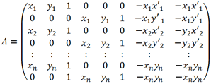
We use the direct linear transformation (DLT) [27] and the least squares method to estimate the homography. Experimentally [1], it has been observed that this approach possesses an outstanding level of accuracy when compared with others. Then, using F and F', we build the matrix A, of 2n × 8 as follows:
 ( 2 )
( 2 )
where the first eight values of H matrix are represented in vector form as hT = (h11,h12,h13,h21,h22,h23,h31,h32) and it is assumed that h33 = 1. Using least squares, the optimal solution h* = (AAT)-1ATp is estimated by applying the pseudo-inverse using the new positions of the feature vector pT = (x'1, y'1,..., x'n, y'n). Thus, h is the homography between the pair of images Ik and Ik+1 . The error of the homography, for a particular feature, is the difference between the true feature positions and the positions predicted in image Ik+1 . That is
x= x'i- x'*i ( 3 )
where x'i is the true feature position and x'*i is the predicted feature position for each displaced feature.
3. IDENTIFICATION OF BACKGROUND AND FOREGROUND FEATURES
When the camera moves, everything in the image seems to move too. In our approach, we analyze the error function density f (x) in each pair of images. Then, given the set of features F, its corresponding set F', the homography matrix H, and assuming that the error density distribution f (x) is Gaussian f (xi) ~ G (xi; mi, si), (this fact is a consequence of the use of the least square method [15]), the classification process that detects static objects is defined as follows:
Let us consider a subset of features G ⊂ F, whose displacement is modeled by a homography H'. The error function x is affected by each element, where the error of the estimated homography h* is affected by
 ( 4 )
( 4 )
where the first term represents the features modeled by H and the second term, those modeled by H'. In the aforementioned assumption, each term has a normal distribution G(pj;x,s). The error mean in (4) is zero, but the individual means of the distributions G(pj;x,s) are displaced, which is a consequence of the mixture of the Gaussians. When the error distribution f (x) is multi-modal, the approaches based on mono-modal distribution selection as seen in [3, 7, 17] are less appealing. If there is more than one predominant displacement in F, each movement H'k is represented by a Gaussian in f(x). We observed that the error function density is well modeled with a mixture of Gaussians as:
f(x)~Sni=1 ai Gi(x; mi,si) , ( 5 )
where ai depends on the amount of elements that conforms each Gaussian. The parameters depend on the number and proportion of eligible features in F. However, for discrete data, it may be convenient to approach it as an incomplete parameter estimation task that can be solved efficiently using the algorithm of expectation maximization (EM) [9]. We then select the homography H for which the probability is largest. That is:
C[f(x)] = E[f(x)], ( 6 )
where C[f(x)] represents the classification function and E[f(x)] is the most probable Gaussian. A new set of features F* is built with the features that belong to the most probable Gaussian for each component. These features correspond to the background. Additionally, one feature xi belongs to the Gaussian Gi, with a probability of 0.95, if it is closer to 2si from the mean mi. New values of h* are obtained by repeating this procedure F←F* until there is a mono-modal distribution. Intuitively, this loop discards the possible outliers resulting from non-static objects, but also miscalculations or unreliable features.
The pseudo-code of this process is shown in Algorithm 1.
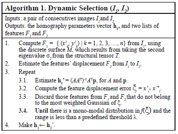
The dynamic selection of feature requires the estimation of the homography elements. The prime condition for estimating the homography induced in the image plane is that AAT be invertible. This constraint is fulfilled if Rank(A) = 8; i.e., if there are at least four non-collinear points. We measure colinearity by fitting a straight line, as in [25]. The residual error magnitude s2 measures the degree of colinearity. For a set of features F in the image Ik, the straight line that best fits the raw data is estimated using Q = P - 1pT, where P is a matrix of 2 × n containing the feature position (xi, yi) for each feature, p = 1/nP1 is the centroid, and 1 is a vector of 1 × n. The factorization of Q by SVD yields Q = SSVT. Here, the second singular value s2 is associated with the null space of QTQv = 0 with vT = (a, b). When s2 is proportionally small, it means that a straight line could geometrically represent the distribution of F. Then, the data dispersion on both orthogonal components must be proportional to the image dimension for reaching a uniform distribution. In other words, if for an image of size n × m, the proportion s2/s1 < n/m holds, then the features are not uniformly distributed and the homography is not reliable.
4. AN APPLICATION: DETECTION OF MOTION
Here we apply the algorithm described for the problem of detecting motion in a camera, motion which is due to vibration.
4.1. Algorithm definition
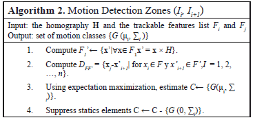
For each pair of consecutive images, Ij, Ij+1, a homography Hj is computed, while Ij+1 is mapped to the initial image I0, using the homographies H*j = H0 × H1 ×...× Hj. The stabilization process is successful when there is a robust estimation of the projection. Using the homography Hj in a pair of images, Ij and Ij+1, the set of features Fj+1, and the features F'j, resulting from the projection of the features Fj via Hj, we have a measure of the error in the estimation of the transformation. The idea is that after the transformation takes place, the feature displacements of fixed objects become approximately zero. We model the displacement distribution DFF' = {xk - x'k | for xk ∈ F and x'I ∈ F'k k = 1, 2, ...,n} , as a mixture of Gaussians f(x) ~ Snl=1 al Gl(ml,Sl), with mean ml and covariance Sl. These parameters are estimated via EM [9]. We assume that the Gaussian Gl(ml,Sl), such that mi ≈ 01×2 corresponds to static areas, while the others correspond to significant trends of motion. Algorithm 2 summarizes this idea.
Finally, Algorithm 3 illustrates the pseudo-code for detecting the motion in cameras subject to vibration.
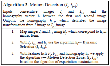
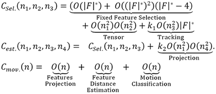
The complexity of the dynamic feature selection strongly depends on the estimation of the structural tensor, which has a complexity of O(n21)O(n22) for a window of n2 × n2, where n2 = 2m + 1. The parameter n1 depends on the image dimensions; e.g., n1 × n1 pixels. The estimation of the homography has a complexity of k1O(n23). The constant k1 depends on either reaching the maximum number of iterations or converging to a minimum error. Each iteration of the algorithm evaluates at least |F|* features, where |F|* is the expected number of these. Then the complexity for each iteration is k1O(n23)|F|*. The feature selection process iterates at the very most |F|*-4 times because of halt constraints. For each iteration, |F|* features are evaluated and the estimation of a homography is performed with a complexity of O(|F|*2). The complexity of the image stabilization process is thus the sum of the complexity of the dynamic selection of features and the complexity of the image projection. The image projection process adds k2O(n2) to the complexity, where k2 = 9. When data needs to be interpolated, the complexity increases to k2(O[n2])(O[m2]), which depends on the window size m. The value of DFF' in the motion detection process has a lineal complexity of n, the number of trackable features in the image. Since it implements the recursive version of EM, the estimation of the number of motion trends has a linear complexity. To sum this up, the complexity of the dynamic selection of features, the image stabilization, and the motion classification is given as:
 (8)
(8)
To detect the numerical system degradation, we use the homography H*j associated with image Ij, a distant homography H*i, associated to image Ii, and the pair of images I'i and I'j, which represents the homography projection of Ii and Ij, respectively. Utilizing the pair of images I'i and I'j, the homography Hij is estimated using Algorithm 1. The homography Hij must satisfy det(Hij) = 1, because Hij has to be the identity matrix. This is so because the projection of Ii into Ij occurs in the same space. When the normalized determinant is not unitary, the system falls into a non-consistent state. Then, when the absolute difference between 1 and det(Hij) is greater than a predefined threshold, the current homography H*j is substituted with H*i'.
5. EXPERIMENTAL RESULTS
The experimental model has two stages. In the first one, we validate the method for the dynamic selection of features. In the second one, we test our method in outdoor environments.
5.1. Algorithm validationThe validation process quantifies the error of the estimated homography for each pair of images. The level of efficiency is measured with root mean square error (RMSE) [2] using the inter-frame selected fixed features. We used two vibration-free image sequences: one of an artificial pattern, and a second of an outdoor scene. A random displacement is applied to both images' sequences to simulate camera vibration.
The artificial pattern consists of a set of square marks of 5 × 5 pixels, uniformly distributed. To simulate the vibration effects, the marks were randomly displaced. These marks correspond to fixed and moving objects. Both groups are displaced with independent random motion. This trial is repeated 100 times for each parameter combination, changing the proportion of moving objects from 10% to 40% with increments of 5%, also changing the amount of displacement from 4 to 14 pixels with increments of two pixels, and using a neighborhood of 4 × 4 pixels. The error is considerably small, even in the cases of large displacements (Figure 1).
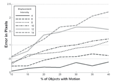
Figure 1. RMSE error of artificial images with additive white noise
The estimated homography error using our approach is small, even when the number of moving features is increased. The feature selection process C[f(x)] is robust because the distribution of fixed objects is identifiably from the error density f(x). Then, using a proportion of motion objects of 40%, with a random displacement intensity of 6 to 14 pixels, and different motion trends from 1 to 5 groups, we observe, as illustrated in Figure 2, that the homography error does not increase considerably, even though there are several trends of motion. This confirms that the criterion for feature detection C[f(x)] is efficient, even when there are several significant motion trends in the objects at the scene.
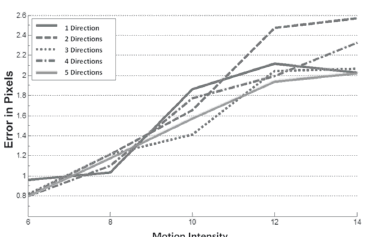
Figure 2. RMSE error images with several moving objects
In a second stage, a sample of 100 vibration-free images was taken from a vehicular intersection. The vibrations were simulated with random displacements in each image. The displacement varies from 2 to 10 pixels with increments of 2 pixels. The neighborhood radio r that surrounds each feature x'I ∈ F is varied from 1 to 5 pixels with increments of one pixel. Note in Figure 3 that the error is significantly higher than in the case of the artificial pattern sequence. The neighborhood size affects the degree of accuracy. Small neighborhoods are more likely not to have enough texture for estimating the feature displacement. In contrast, in large neighborhoods, there is the risk of selecting regions that are part of objects moving in different directions. However, the results show that our approach is capable of estimating, with a high degree of accuracy, the image transformations in a controlled environment.
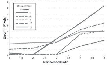
Figure 3. RMSE graph error from a short image sequence used to validate our approach
5.2. Outdoor environment
Then, we applied our method in two different scenarios. Table 1 summarizes the main characteristics of each scenario. The sequence of images from the intersection shows changing luminance and motion conditions. The objects with motion include vehicles, bicycles, and pedestrians. In several instances, the sequence of images has vibrations due to vehicles, rain, and wind. The freeway sequence has poor video quality and a high zoom level which increments the effect of the perceived vibration. Figure 4 shows the number of features found and selected for each of the test sequences. From the amount of features, seen as blue lines, it was determined that those remaining fixed, seen as green lines, were useful, discarding those that present movement and could not be tracked-seen as red lines. The changes in luminance, reflection, and the effects of rain, cloud occlusions, and compression level, have an impact on the detected number of fixed features. Figures 5 and 6 show representative situations for each sequence. Even though, there are clearly detectable trends of motion, the distribution of texture is non-uniform, and there are changes of luminance due to rain and light reflection, as is noted in Figure 5. Overall, considering the poor quality of the video, which is the first image of Figure 6, fixed and moving features were detected efficiently as can be seen in Figure 5. The sudden illumination changes and reflections are supported efficiently. When the features are insufficient or are not uniformly distributed for estimating the parameter of the homography, the reliability measure provides a criterion for deciding whether the homography transformation is satisfactory. Figure 6 illustrates this case. In the first image, the proportion of eigenvalues taken from the feature distribution is 0.6113, which is close to the ideal proportion of images sizes (242/360 = 0.6722). In contrast, in the second case, this proportion is 0.2846. This condition warns the method that there is a lack of information to distinguish between moving and static objects.
Table 1. Some parameters of the image sequences.
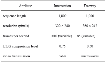
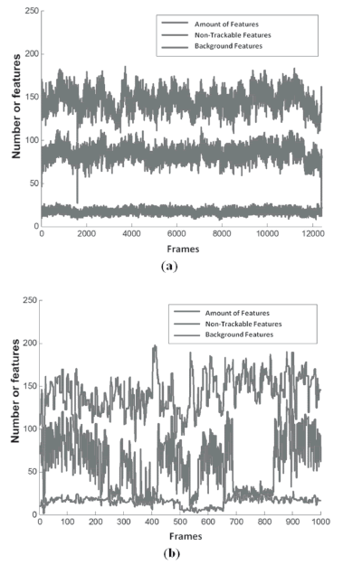
Figure 4. Evolution of trackable features over time. In (a), we illustrate the results for the intersection sequence and in (b), the results for the freeway sequence
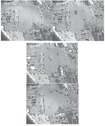
Figure 5. Motion detection vibration caused by rain and wind
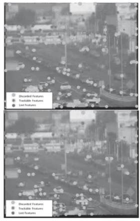
Figure 6. Frames with/without an adequate distribution of trackable features in poor quality video sequences
When the regions containing moving objects are larger than those containing static objects, the algorithm cannot distinguish between them because there is not enough information in the error function f(x). In Figure 7, we illustrate a scenario where it is not possible to detect background features. In this Figure, blue arrows illustrate the main trends of vehicular motion. In Figure 7(a), the estimated Gaussians of f(x) is shown. It is noteworthy that there is not enough texture in the background to select features. To solve this problem, we have two possible existing options. The first consists of replacing the classification function C[f(x)] and incorporating additional information about the scenario. The second option consists of selecting image regions with static features.
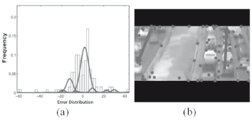
Figure 7. Non-supported scenarios. In (a), the distribution is not conveniently modeled with a mixture of Gaussians. In (b) there is not enough texture information in the static regions
6. CONCLUSION
In this investigation, we introduced a method to efficiently detect motion patterns in cameras subject to vibration, a method which is based on the dynamic selection of features. The method gave satisfactory results in both artificial and outdoor scenarios. The use of dynamic features and the proposed selection criterion resulted in an efficient and adaptable algorithm for coping with scene changing conditions such as illumination, occlusions, and poor video quality. The numerical degradation stage helped to boost the algorithm performance for extended sequences, providing spatial consistency. Our approach is efficient and adaptable to different environmental conditions, without affecting motion detection efficiency.
ACKNOWLDGEMENTS
We express our gratitude to the anonymous reviewers of this work. This work was supported by the Consejo Nacional de Ciencia y Tecnología under grant No. 25288, the Fulbright Scholarship Board, and the Instituto Politécnico Nacional under grant No. 20110705.
REFERENCES
[1] Agarwal, A., Jawahar, C.V. and Narayanan P.J., A Survey of Planar Homography Estimation Techniques, Tech. Report, International Institute of Information Technology Hyderabad, 2005. [ Links ]
[2] Anderson, M. and Woessner, W., Applied Groundwater Modeling: Simulation of Flow and Advective Transport, Academic Press, 1992. [ Links ]
[3] Censi, A., Fusiello, A., and Roberto, V. Image Stabilization by Features Tracking. International Conference on Image Analysis and Processing, 665 - 667, 1999. [ Links ]
[4] Cham, T. and Rehg, J., Dynamic Feature Ordering for Ef?cient Registration, IEEE ICCV, Vol. 2, pp.1084, 1999.
[5] Chen, L., Armstrong, C.W. and Raftopoulos D.D., An Investigation on the Acurracy of Three-Dimensional Space Reconstruction using the Direct Linear Transformation Technique, Journal of Biomechanics, Vol. 27, No. 4, 493-500, 1994. [ Links ]
[6] Chen, H., Liu, T. and Fuh, C., Probabilistic Tracking with Adaptive Feature Selection, IEEE ICPR, Vol. 2, 736-739, 2004. [ Links ]
[7] Chum, O. and Matas, J., Optimal Randomized RANSAC, IEEE TPAMI, (8), 1472-1482, 2008. [ Links ]
[8] Collins, T. and Yanxi, L., On-Line Selection of Discriminative Tracking Features, IEEE TPAMI, 27(10), pp. 1631 - 1643, 2005. [ Links ]
[9] Dempster, A., Laird, N., and Rubin, D. Maximum Likelihood from Incomplete Data via the EM Algorithm, Journal of the Royal Statistical Society, No. 1, 1-38, 1997. [ Links ]
[10] W. Eadie, D. Drijard, F. James, M. Roos, and B. Sadoulet, Statistical Methods in Experimental Physics. Amsterdam: North-Holland, 1971. [ Links ]
[11] Fischler, M. and Bolles, R., Random Sample Consensus: A Paradigm for Model Fitting with Applications to Image Analysis and Automated Cartography, ACM Proceedings on Communication, Vol. 24, 381-395, 1981 [ Links ]
[12] Gil, S., Feature Selection for Object Tracking in Traffic Scenes, Technical Report on International Computer Science Institute, tr-94-060, 1994. [ Links ]
[13] Jurisica, L., Hubinský, P., and Knot, J., Feature Based Object Tracking for Oscillation Detection, International Conference of Radioelecktronika, 316-319, 2006. [ Links ]
[14] Kalman, R.A New Approach to Linear Filtering and Prediction Problems, Journal of Basic Engineering, No. 1, 35-45, 1960. [ Links ]
[15] Kariya, T. and Kurata, H., Generalized Least Squares, Wiley, 2004. [ Links ]
[16] Kim Z., Real Time Object Tracking Based on Dynamic Feature Grouping with Background Subtraction, IEEE CVPR, 1-8, 2008. [ Links ]
[17] Lacey, A., Pinitkarn, N., and Thacker, N.,An Evaluation of the Performance of RANSAC Algorithms for Stereo Camera Calibration. BMVC, 2000. [ Links ]
[18] Lucas, B. and Kanade, T., An Iterative Image Registration Technique with an Application to Stereo Vision. DARPA Proceedings on Image Understanding Workshop, 674-679, 1981. [ Links ]
[19] Mikolajczyk, K. and Schmid, C. A Performance Evaluation of Local Descriptors. IEEE TPAMI, 2005, vol. 27, 1615-1630. [ Links ]
[20] Shi, J. and Tomasi, C., Good Features to Track. IEEE CVPR, 593-600, 1994. [ Links ]
[21] Soille, P., Morphological Image Analysis: Principles and Applications. Springer-Verlag, 1999. [ Links ]
[22] Tang, F. and Tao, H., Object Tracking with Dynamic Feature Graph, Workshop on Visual Performance Evaluation of Tracking and Surveillance, 25-32, 2005. [ Links ]
[23] Tomasi C., Input Redundancy and Output Observability in the Analysis of Visual Motion. Proceedings of the Sixth International Symposium on Robotics Research, 213-222, 1993. [ Links ]
[24] Tomasi, C., Mathematical Modeling of Continuous Systems. Duke University, 2004. [ Links ]
[25] Wald, A. Sequential Tests of Statistical Hypotheses, Annals of Mathematical Statistic, Vol. 16. No. 2, 117-186, 1945. [ Links ]
[26] Yilmaz, A., Javed, O. and Shah, M., Object Tracking: A Survey, ACM Computer Surveys, 38(4), 13+, 2006. [ Links ]


