


Serviços Personalizados
Journal
Artigo
 Inglês (pdf)
 Artigo em XML
 Referências do artigo
 Enviar este artigo por email
Indicadores
-
 Citado por SciELO
 -
 Acessos
Links relacionados
-
 Citado por Google
 -
 Similares em
SciELO
Similares em
SciELO -
 Similares em Google
Compartilhar

 Permalink
DYNA
versão impressa ISSN 0012-7353
Dyna rev.fac.nac.minas vol.79 no.176 Medellín nov./dez. 2012
A PROCEDURE TO CALIBRATE AND PERFORM THE BENDER ELEMENT TEST
UN PROCEDIMIENTO PARA CALIBRAR Y EJECUTAR EL ENSAYO BENDER ELEMENT
JAVIER FERNANDO CAMACHO-TAUTA
PhD, Profesor Asociado, Universidad Militar Nueva Granada, javier.camacho@unimilitar.edu.co
JUAN DAVID JIMÉNEZ ÁLVAREZ
Estudiante de Ing. Civil, Universidad Militar Nueva Granada, u1100849@unimilitar.edu.co
OSCAR JAVER REYES-ORTIZ
PhD, Profesor Titular, Universidad Militar Nueva Granada, oscar.reyes@unimilitar.edu.co
Received for review January 19th, 2012, accepted June 20th, 2012, final version July, 11th, 2012
ABSTRACT: The bender element (BE) test method is used in a laboratory to obtain the shear wave velocity of soils. Despite its apparent simplicity, there is still no standard for this test. A number of factors affect the reliability of the results. These factors are taken into account to design and build a BE system in a triaxial cell. A method for calibrating the system is proposed, using aluminum rods of different lengths. Recommendations are made regarding the selection of the frequency of the pulse used to produce the perturbation for carrying out the test. Finally, a series of tests carried out on two kinds of sand specimens are presented.
KEYWORDS: bender element, shear modulus, shear wave velocity
RESUMEN: El método de ensayo bender element es utilizado en laboratorio para obtener la velocidad de la onda cortante de suelos. A pesar de su aparente simplicidad, aún no existe una norma para este ensayo. Existen factores que pueden tener alguna incidencia sobre el resultado. Estos factores son tenidos en cuenta para diseñar y construir un sistema de ensayo en una cámara triaxial. Se propone un método para calibrar el sistema mediante la utilización de barras de aluminio de diferente longitud y se hacen recomendaciones para la ejecución del ensayo, en lo relacionado con la selección de la frecuencia del pulso sinusoidal utilizado para producir la perturbación. Finalmente, se presentan ensayos efectuados sobre dos muestras de arena.
PALABRAS CLAVE: bender element, módulo cortante, velocidad de onda cortante
1. INTRODUCTION
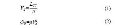
Bender element (BE) testing has appeared as one promising way to obtain shear modulus at small strains [1]. A voltage signal is applied to a piezoceramic element, which transmits a small shearing movement over one end of the cylindrical soil specimen. This disturbance travels along the specimen until the other end where a similar element receives the mechanical perturbation and generates a voltage [2]. The signal travels a distance between elements (LTT) and the time difference between the emitted and received signals represents the time of the propagation of the signal (tt). These measurements enable one to compute the shear wave velocity (VS) and the initial shear modulus (G0) of a specimen with a known soil mass density (r):
The BE system is installed in a geotechnical device capable of providing control and the measurement of stress and/or strain on the soil specimen. The use of BE in laboratory research equipments has increased during recent years. The equipment includes: oedometers, direct shear devices, triaxial cells, cyclic triaxial apparatuses, stress-path cells, resonant-column, centrifuges, hollow cylinders, calibration chambers, and true triaxial cells [3].
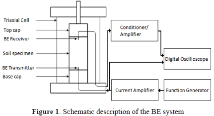
This paper shows the implementation of a BE system in a triaxial cell as illustrated in Fig. 1. The implementation takes into account the main factors that could influence the operation of the test. A calibration procedure is proposed and conducted to assure the satisfactory performance of the system. Finally, a series of tests carried out on two kinds of sands are presented.
2. OPERATING PRINCIPLE OF A BE SYSTEM
A BE system supports its operation in the piezoelectric property, which allows for the generation and detection of small shear waves travelling in a soil specimen. Electronic peripherals permit the generation, acquisition, and storing of input and output signals. Software tools for data analysis are used to derive the soil properties from the raw data.
A BE is composed of two thin piezoceramic plates cross-sectionally polarized and firmly bonded together. The orientation of the polarization can be in the same or in an opposite direction. A pair composed by two elements with polarization oriented in the same direction and wired in such way that the supply voltage is applied or measured to each layer individually, is called a parallel BE (Fig. 2a). This arrangement is more adequate when the BE works as a source. A source is defined as the transducer that transforms electrical energy into mechanical energy (the transmitter of motion waves).
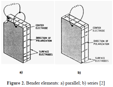
A pair composed of two elements with polarization oriented in the opposite direction operates in a series (Fig. 2b). The voltage is the sum of the individual voltages of each element. This configuration is adequate for the purposes of generation, converting mechanical energy into electrical energy, that is, it works as a receiver of the wave motion.
When voltage is applied, the polarization of the ceramic material and the type of electrical connections permit the elongation of one element and the shortening of the second element. The result is a bending displacement [2]. If inserted properly into a soil, the bending displacement of the BE produces a perturbation with a strong shear wave content.
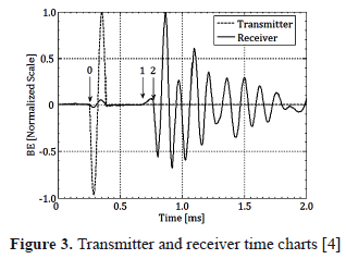
Figure 3 shows an example of the BE response in which a single sinusoidal pulse has been used to excite the BE transmitter, and the response of the BE receiver is presented on the same graph. The travel time is obtained by measuring the lapse between the instant the wave starts to propagate (point 0) into the soil up to its arrival at the BE receiver (point 2).
Initially, researchers used a step signal (square wave with very low frequency) to excite the BE transmitter, not only because the starting time was easily defined, but also because the sudden change produces a significant perturbation. Nevertheless, the step signal produces an output composed of all frequencies [5]. Over the course of many years, researchers have consistently shown preference for a sine pulse as demonstrated by an international parallel test on the measurement of G using bender elements [6].
3. FACTORS AFFECTING THE ACCURACY OF BE TESTING
The wave propagation in BE testing has been widely studied, both theoretically and experimentally. Several factors influence the reliability of this testing method, such as the near-field effect [7-11]; directivity [11]; travel distance [8]; incidence of boundaries [9]; sample geometry and size [12,13]; and crosstalk [3,11]. Such factors can be grouped into the following categories: the quality of manufacturing and installation; the coupling and alignment of BE into the specimen; and the near-field and specimen size effects.
3.1. Manufacturing and installation of BE
Polarization and wiring should be accurately performed in order to avoid abnormal performance. The adequate shielding of layers and grounded transducers can reduce the crosstalk effect [11]. Crosstalk is the reception of a quasi-simultaneous response, usually with a similar shape, to the input signal that could obscure the first arrival of shear waves. Grounding can be improved by coating the transducer with a conductive silver paint over the insulating epoxy resin [14]. Leak-free connections can increase the signal-to-noise ratio, reducing the testing time and avoiding the needing to clean the signal by using filtering methods [15].
3.2. Coupling and alignment of BE
Coupling between BE and soil is essential to ensure the effective transference of energy between them. The method of introducing the BE into the soil varies depending of its stiffness. The procedure chosen must satisfy: (i) good coupling, (ii) low alteration of the surrounding soil, and (iii) preservation of the integrity of the transducers.
For weak soils, protrusion with pressure is acceptable. Excavation of undersized slots and protrusion is used for stiff clays. These slots should be excavated with high precision in order to have a minimum distance between the elements and the soil. The excavation of oversized slots and sealing is applicable for cemented sands [15].
The transmitter and receiver are aligned when they share the same plane. Misalignment increases the possibility of contamination with other indirect waves and of receiving weak direct shear waves produced by the transmitter [16]. Top and base caps should have marks that are clear in order to align the transducers properly.
3.3. Near-field effect
The notion of the near-field effect in geotechnics was first studied in cross-hole tests [7]. The near-field effect is responsible for the common difficulty in the identification of the arrival time of shear waves. In the fundamental solution for transverse equations of motion of shear waves, three components appear: two of them propagate at shear-wave velocity while the third propagates at compression-wave velocity. These three components attenuate at different rates: faster waves attenuate earlier than others. The near-field effect has an important contribution close to the source and therefore if the receiver is too close to the transmitter, the arrival of the shear wave is masked by this effect. This undesirable effect can be minimized by increasing the frequency (f) of the shear wave, which in turn increases the ratio between the travel distance (LTT) and the wavelength (λ) [17]. A range of 2< LTT/λ<9 is recommended [7,9,10,18-20].
3.4. Effects of the specimen size
Reflections of waves at boundaries could be the main factor which generates the observed complexity of the arrival trace [3]. Distances between the source, boundaries, and receiver, as well as the location of source and receiver relative to the boundaries, have great importance in the acquisition of the signal.
The sample size could produce [21]: (i) effects introduced by end rebounds which provoke interferences and signal overlap; and (ii) effects due the cylindrical boundary that produce an interfered signal where each frequency travels at a different velocity especially when wavelengths are comparable with the size of the specimen. A set of simulations by means of an explicit finite difference method allowed to find that the best results are obtained for slenderness ratios greater than 2 [22]. Other studies agree with this estimation [9,10,19]. Specimens with small diameters are more affected by reflections from lateral boundaries [13].
4. DIFFERENCES BETWEEN INPUT AND OUTPUT SIGNALS
In theory, if the transmitter and receiver are in direct contact (i.e., no specimen is located between the transducers) and the transmitter is excited with a specified function, the receiver should record a similar waveform. However, the generated waveform that is effectively induced into the soil to be tested is generally different due to a number of factors. As product of those factors, four characteristics summarize the differences between input and output signals: magnitude, time delay, polarity, and shape.
4.1. Magnitude
The magnitude of the output signal depends on various facts, including: (i) the transformation efficiency of the piezoelectric transducers (mechanical to electrical at the BE transmitter, and electrical to mechanical at the BE receiver); (ii) the type of connection between electrodes, namely serial or parallel, (iii) the quality of the contact between BE tips and soil; and (iv) the gain of the amplifier. The magnitude of the output signal is not critical to the interpretative processes; the only mandatory condition is to have enough resolution to differentiate the characteristic points of the waveform.
4.2. Time delay
Usually, the travel time in electronic equipment, cables, and connections is assumed to be zero. This time delay can be considered to be a constant of the system that has to be subtracted from the total travel time measured during a test.
4.3. Polarity
Because the output of the BE receiver is an electrical tension, its sign depends on the wiring of the BE receiver. This effect is called polarity: if the wiring is inverted, a positive signal applied to the BE transmitter produces a negative signal on the BE receiver. The signal is not distorted, but the user should take into account this change in polarity in order to avoid an erroneous identification of the arrival time.
4.4. Shape
The shape of the output signal depends on a more complex phenomenon not only due to the BE receiver but also to the BE transmitter. According to laser measurements [22,23] and measurements with miniature accelerometers [4,24], the actual movement of the BE transmitter is different from the input signal. Specific characteristics of the signal may introduce additional changes in the shape. For example, a transient function like a pulse is more difficult to follow using the BE due to the inertia effect. Finally, the propagation of the wave transforms the frequency content of the signal depending on the characteristics of the medium. Consequently, the signal that arrives at the receiver is different from the one in the transmitter.
5. INTERPRETATION OF BE TESTS
The principle of BE testing is simple; however a clear identification of the arrival time is not always possible, frequently being a complex issue. Even to the present day, there is no specialized technique with an adequate level of accuracy and reproducibility to be adopted as the standard. Many studies have been made and a number of testing and interpretation methods have been proposed. The interpretation methods can be grouped in two main categories: time domain and frequency domain [25]. In this paper, time domain analysis is used.
Time domain analysis is referred to as an analysis made from signals represented along the axis of time in which the input and/or output waveforms are plotted. Two points of these plots can be selected following a given criterion, where their time difference is defined as the travel time between the transmitter and the receiver of the wave under analysis [26]. Estimation of the travel time by the identification of the first direct arrival in the output signal was the initial assumption in this method (time difference between points 0 and 1 in Fig. 3). This assumption is an intuitive interpretation following the method used on in situ geophysical measurements and was the interpretation method initially adopted [1,2,27]. The method remained unchanged for nearly 10 years until a travel-time determination based on the first inversion (point 2 in Fig. 3) of the received signal was proposed [28].
6. EXPERIMENTAL PROCEDURE
6.1. Equipment
A triaxial cell is equipped with a set of BE manufactured by the University of Western Australia [29]. The cell pressure is controlled by a pneumatic system with a maximum confinement 700 kPa and a precision of 10 kPa. The specimens are 14 cm in height and 7 cm in diameter on average. The size and proportions are in agreement with the suggestions of previously-reported works.
The transmitter and receiver are located at the base cap and top cap of the triaxial device, respectively. The input signal is generated by a function generator (RIGOL, DG1022). A current amplifier stabilizes the signal and send it to the BE transmitter. The output signal of the BE receiver is amplified and both input and output signals are collected by a digital oscilloscope (Tektronics, 3S2012B). A vertical transducer is used to measure any variation of the specimen height. Figure 1 shows a schematic of the system.
6.2. Calibration
The verification of polarity was done using a single-sine pulse and BE located in direct tip-to-tip contact. Once the polarity was determined, the wiring was adjusted in order to obtain positive polarity, avoiding making corrections during post processing.
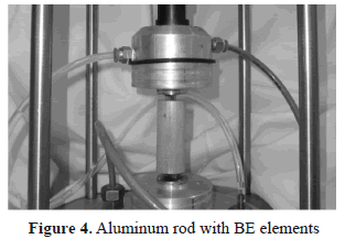
A procedure to assess the equipment time delay is presented as follows: an aluminum rod is placed between the pair of BE in contact with their tips (Fig. 4). Despite the poor coupling between the rod and BE, the transmitter is able to produce a perturbation on the rod. The receiver on the other end of the rod detects the arrival, and the total travel time is measured. Aluminum rods of different length allow for one to measure the travel time (tt) of the shear wave for various travel distances (LTT). The intersection with the horizontal axis in Figure 5 is the time delay and the slope is the shear-wave velocity. The time delay (15ms) should be included in the computation of the shear modulus. For typical soil properties, the omission of this correction can produce lower computed values of about 8%.
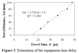
The shear wave velocity in aluminum is a well-established property (3150 m/s) [30]. Thus, the slope of the graph should exhibit a similar value. According to the trend line shown in Fig. 5, the estimated shear wave velocity in aluminum was 2911 m/s. The difference between the measured and theoretical velocities is 7.5%. The dispersion could indicate that it is being influenced by other waves either directly or through reflections on the surface of the rod. This influence is a result of a complex process which can reduce one's ability to interpret the arrival of shear waves.
6.3. Preparation of specimens
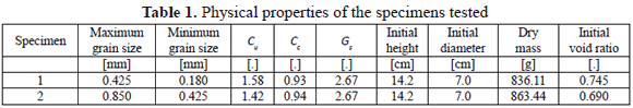
Two specimens of alluvial sand were prepared by the dry deposition method [31]. Table 1 shows the physical properties of the two specimens. Both sands exhibit similar uniformity (Cu) and curvature (Cc) coefficients, and the same specific gravity of solids (Gs), but the gradation of specimen 1 is finer than specimen 2's.
The sand was introduced into the oven for 24 h to remove any trace of initial moisture. Once the material cooled, it was weighted to verify constant weight after 2 consecutive drying cycles. According to the specimen dimensions, the soil mass was separated and divided into 5 equal portions.
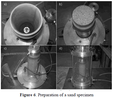
The membrane and two o-rings were located in the base pedestal and a split mold was placed on it to accommodate the membrane. A vacuum pump was used to force the membrane to stick to the mold, becoming the cylindrical shape of it.
The soil was carefully poured into the interior of the membrane using a funnel. During the pouring, the funnel was moved along the circular section maintaining a constant height. Each layer was compacted and capped with a piston. The final height of each layer was verified with a caliper in order to guarantee the void ratio previously defined. The process was repeated for the next 4 layers.
The top cap was carefully placed on the unit and the membrane was accommodated to cover the top cap and two o-rings; 20 kPa of vacuum were applied onto the interior of the specimen and the mold was removed. Immediately afterwards, the chamber was placed in position and filled with water. Finally, the vacuum was gradually replaced by cell pressure according to the triaxial stress condition required to perform BE tests. Figure 6 shows some aspects of the process.
6.4. BE tests
Each specimen was tested under dry conditions and subjected to 50, 100, 200, and 400 kPa of isotropic cell pressures. In principle, the shear waves do not travel in water and therefore humidity does not interfere with the propagation velocity of these waves. In each stress condition, the following procedure was conducted:
- The function generator is programmed to produce a linear sine sweep signal with frequency content between 1-20 kHz, for a total duration of 40 ms, and at an amplitude of 20 Vpp. This signal is sent to the BE transmitter.
- The digital oscilloscope acquires both input and output signals. The Fast Fourier Transform (FFT) computed in real time by the oscilloscope allows one to identify the specific frequency in which the response of the BE receiver is higher.
- The function generator is turned to single-sine pulse mode with the frequency previously determined. The period of the signal is selected in order to allow enough time for the attenuation of the BE response before the next pulse.
- With the sine pulse, the input and output signals of a number of pulses are stacked in order to cancel out random noise, obtaining a clean response from the BE receiver.
- The arrival time is identified by the first inversion method. The travel time is the difference between the arrival time and the time at the start of the sine pulse. Then, the equipment time delay is subtracted from the last result.
- The travel distance is the tip-to-tip length, which is the height of the specimen minus the length of each BE.
- The shear-wave velocity and the shear modulus are computed by (1) and (2), respectively.
- The wavelength λ = VS/f is computed, and the ratio LTT/λ>2 is checked.
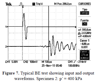
Figure 7 shows a typical screen of the oscilloscope in the BE test. Channel 1 exhibits the single-sine pulse use to excite the BE transmitter and Channel 2 shows the output signal acquired by the BE receiver. Vertical cursors indicate the initial and arrival times used to compute the travel time.
7. RESULTS AND DISCUSSION
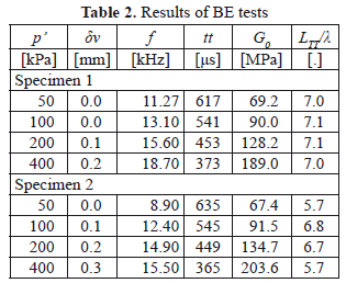
The testing procedure described above was performed for both sand specimens and confinements from 50 to 400 kPa. Table 2 shows the raw data and computed results of the BE tests including the verification of the adequate travel distance-to-wavelength ratio that minimize the near-field effect. dv is the axial deformation of the specimen due to confinement.
Shear moduli obtained by the BE tests were compared with (3) [32]:
Where A and m are experimental factors obtained by curve fitting. Equation (3) does not have dimensional homogeneity; hence numeric values of parameters A and m depend on the unit system used. The results of these parameters are presented in Fig. 8. Experimental results are in good agreement with the form of (3) as can be confirmed by the determination coefficients, which were greater than 0.99.
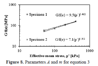
A compilation of many test results shows that m varies between 0.4-0.5, and A fluctuates between 7.0-14.1 for G and p' expressed in MPa and kPa, respectively [4]. The relations of these parameters with physical properties of the sands are not well established. The sands tested are very similar; the only difference is the grain size, which nevertheless is in the same order of magnitude. The results of this paper could suggest that the finer the sand, the greater parameter A will be. Moreover, confinement has more influence on coarse sands. This trend may be due to the number of intergranular contacts and their increase with confinement.
8. CONCLUSIONS
A BE system was designed and built using equipment of relatively low cost, but taking in to account the main recommendations found in the literature review.
The proposed calibration method using aluminum rods of various lengths is an effective and reliable way for obtaining the equipment time delay.
BE testing is still controversial because of the need for user judgment. The recommended procedure presented in this paper seeks for a reduction of subjectivity. The procedure uses the single-sine pulse as input signal according to the suggestions of many researchers, but the frequency of this pulse is selected following two criteria: firstly, to obtain a maximum response of the system in order to get a clear output; secondly, to assure that the travel length-to-wavelength ratio is high enough to reduce near-field and specimen size effects.
ACKNOWLEDGEMENTS
This paper is a result of the Research Projects PIC ING-811 and ING-723 supported by the Nueva Granada Military University. Eng. Germán Castañeda designed and manufactured the electronic compounds.
REFERENCES
[1] Shirley, D. J. and Hampton, L. D., Shear-wave measurement in laboratory sediments, J Acoust Soc Am, 63, pp. 607-613, 1978. [ Links ]
[2] Dyvik, R. and Madshus, C., Lab measurements of Gmax using bender elements, Proc, ASCE Annual Convention on Advances in the Art of Testing Soils under Cyclic Conditions, Detroit, Michigan, pp. 186-196, 1985. [ Links ]
[3] Ferreira, C., The use of seismic wave velocities in the measurement of stiffness of a residual soil [PhD Thesis], Porto: University of Porto, 2008. [ Links ]
[4] Camacho-Tauta, J., Evaluation of the small-strain stiffness of soil by non-conventional dynamic testing methods [PhD Thesis], Lisbon: Technical University of Lisbon, 2011. [ Links ]
[5] Bray, J. D., Riemer, M. F. and Gookin, W. B., On the dynamic characterization of soils, Proceedings of the Second International Conference Earthquake Geotechnical Engineering, Lisbon, 2003. [ Links ]
[6] Yamashita, S., Kawaguchi, T., Nakata, Y., Mikami, T., Fujiwara, T. and Shibuya, S., Interpretation of international parallel test on measurement of Gmax using bender elements, Soils and Foundations, 49, pp. 631-650, 2009. [ Links ]
[7] Sanchez-Salinero, I., Roesset, J. M. and Stokoe, K. H. I., Analytical studies of body wave propagation and attenuation [Report GR 86-15], Austin: University of Texas, 1986. [ Links ]
[8] Brignoli, E. G., Gotti, M. and Stokoe, K. H. I., Measurement of shear waves in laboratory specimens by means of piezoelectric transducers, Geotechnical Testing Journal, ASTM, 19, pp. 384-397, 1996. [ Links ]
[9] Arulnathan, R., Boulanger, R. W. and Riemer, M. F., Analysis of bender element tests, Geotechnical Testing Journal, ASTM, 21, pp. 120-131, 1998. [ Links ]
[10] Arroyo, M., Muir Wood, D. and Greening, P. D., Source near-field effects and pulse tests in soils samples, Géotechnique, 53, pp. 337-345, 2003. [ Links ]
[11] Lee, J.-S. and Santamarina, J. C., Bender elements: performance and signal interpretation, Journal of Geotechnical and Geoenvironmental Engineering, ASCE, 131, pp. 1063-1070, 2005. [ Links ]
[12] Rio, J., Greening, P. and Medina, L., Influence of sample geometry on shear wave propagation using bender elements, Deformation Characteristics of Geomaterials, Lyon, pp. 963-967, 2003. [ Links ]
[13] Arroyo, M., Muir Wood, D., Greening, P. D., Medina, L. and Rio J., Effects of sample size on bender-based axial G0 measurements, Géotechnique, 56, pp. 39-52, 2006. [ Links ]
[14] Brocanelli, D. and Rinaldi, V., Measurement of low-strain material damping and wave velocity with bender elements in the frequency domain, Canadian Geotechnical Journal, 35, pp. 1032-1040, 1998. [ Links ]
[15] Jovicic, V., Conditions for rigorous bender element test in triaxial cell, Proceedings of the workshop on current practices of the use of bender element technique, Lyon, France, 2003. [ Links ]
[16] Gohl, W. B. and Finn, W. D. L., Use of piezoceramic bender elements in soil dynamics testing, Proceedings of ASCE National Convention, Recent Advances in Instrumentation, Data Acquisition and Testing in Soil Dynamics, Florida, Geotechnical Special Publication, 29, pp. 118-133, 1991. [ Links ]
[17] Gordon, M. A. and Clayton, C. R. I., Measurements of stiffness of soils using small triaxial testing and bender elements, In: Modern Geophysics in Engineering Geology (MCCANN D. M., EDDELSTON M., FENNING P. J. and REEVES G. M., eds.). Geological Society Engineering Geology Special Publication, pp. 365-371, 1997. [ Links ]
[18] Gajo, A., Fedel, A. and Mongiovi, L., Experimental analysis of the effects of fluid-solid coupling on the velocity of elastic waves in saturated porous media, Géotechnique, 47, pp. 993-1008, 1997. [ Links ]
[19] Pennington, D. S., Nash, D. F. T. and Lings, M., Horizontally-mounted bender elements for measuring anisotropic shear moduli in triaxial clay specimens, Geotechnical Testing Journal, ASTM, 24, pp. 133-44, 2001. [ Links ]
[20] Wang, Y. H., Lo K. F., Yan, W. M. and Dong, X. B., Measurement biases in the bender element test, Journal of Geotechnical and Geoenvironmental Engineering, ASCE, 133, pp. 564-574, 2007. [ Links ]
[21] Arroyo, M., Pulse tests in soils samples [PhD Thesis], Bristol: University of Bristol, 2001. [ Links ]
[22] Rio, J., Advances in laboratory geophysics using bender elements [PhD Thesis], London: University of London, 2006. [ Links ]
[23] Pallara, O., Mattone, M. and Lo Presti D. C. F., Bender elements: bad source - good receiver, Deformational Characteristics of Geomaterials, Atlanta, 2, pp. 697-702, 2008. [ Links ]
[24] Camacho-Tauta, J., Cascante, G., Santos, J. A. and Viana Da Fonseca, A., Measurements of shear wave velocity by resonant-column test, bender element test and miniature accelerometers, 2011 Pan-Am Geotechnical Conference, Toronto, 2011. [ Links ]
[25] Viana Da Fonseca, A., Ferreira, C. and Fahey, M., A framework interpreting bender element tests, combining time-domain and frequency-domain methods, Geotechnical Testing Journal, ASTM, 32, pp. 1-17, 2009. [ Links ]
[26] Franco, E. E., Mesa, J. M. and Buiochi, F., Measurement of elastic properties of materials by the ultrasonic through-transmission technique, Revista Dyna, 168, pp. 59-64, 2011. [ Links ]
[27] Shirley, D. J., An improved shear wave transducer, J Acoust Soc Am, 63, pp. 1643-1645, 1978. [ Links ]
[28] Viggiani, G. and Atkinson, J. H., Interpretation of bender element tests, Géotechnique, 45, pp. 149-154, 1995. [ Links ]
[29] Ismail, M., Sharma, S. S. and Fahey, M. A., small true triaxial apparatus with wave velocity measurement, Geotechnical Testing Journal, ASTM, 28, pp. 113-122, 2005. [ Links ]
[30] Ross, R. B., Metallic materials specification handbook, Spon, London, 1980. [ Links ]
[31] ISHIHARA, K. Soil behaviour in earthquake geotechnics, Oxford Science Publications, 1996. [ Links ]
[32] Iwasaki, T. and Tatsuoka, F., Effects of grain size and grading on dynamic shear moduli of sands, Soils and Foundations, 17, pp. 19-35, 1977. [ Links ]
