


 Inglês (pdf)
 Artigo em XML
 Referências do artigo
 Enviar este artigo por email
 Citado por SciELO
  Citado por Google
  Similares em
SciELO
Similares em
SciELO  Similares em Google
 Permalink
1. Introduction
The measurement of electromagnetic fields generated by lightning has been carried out in the last four decades and consequently many features of the phenomenon have been revealed. A major part of these works was conducted using sensors to measure the radiated electric or magnetic fields generated by cloud-to-ground (CG) lightning flashes [1].
The knowledge of the electric fields produced by lightning (LEF) is important to: (a) identify some parameters of lightning flashes (multiplicity, flash duration, interstroke intervals and currents); (b) understand the discharge mechanism and physical discharge processes; (c) design lightning protection systems; (d) lightning location networks; (e) determine the electromagnetic compatibility requirements of equipment and systems [1-4].
Due its importance, lightning characterization using LEF measurements has been developed in several regions of the world. In fact, lightning location networks, detection and warning systems, lightning flash density estimations and indirect determination of lightning current amplitudes are successful applications of indirect measurements of LEF. In addition, the measurement of these fields allows establishing relationships between lightning flash events and transients that could help in the classification of electromagnetic disturbances [5].
To develop and evaluate models of the lightning return stroke and determine the lightning current features, it is necessary to determine, in a reliable way, various temporal features of the electric field waveforms such as: the peak value, rise-time, zero-crossing time, slow-front and fast-front duration, and peak value of the electric field derivative [6-8] [6-8]. However, the extraction of lightning parameters from LEF or current measurements is not a simple task due to the presence of noise in the recorded signals, mainly caused by the measuring system itself and other undesired components present in the electromagnetic environment [7-9].
In the past, noise removal from LEF signals has been achieved using low-pass filters (hardware) and digital filters based on the discrete Fourier transform (software), both methods with cut-off frequencies ranging from 200 kHz to 30 MHz [9,10]. However, these methods may affect part of the original signal, causing loss of information. To overcome this problem, some denoising techniques based on time, frequency or hybrid time-frequency domains have been proposed in the last two decades.
The conventional Fourier transform (FT) and the short-time Fourier transform (STFT) were the first approaches to reduce the noise on lightning electric field signatures [11]. Because of the limitations of FT and STFT (loss of resolution in time or frequency), new signal processing methods have been proposed. Wavelet transform (WT) has been used for different purposes in the study of lightning activity, including noise reduction and frequency anlaysis [3,8,12]. The major disadvantages of WT are the complexity of calculations, the sensitivity to some noise levels, and the dependence of its accuracy on the selected wavelet base (mother) function [8,12].
Recently, noise reduction methods on LEF signals have been extended to the application of the discrete fractional Fourier transform (DFRFT) [13,14]. However, it is not possible to have a desired signal because, by nature, the LEF have a random behavior and the waveforms change with respect to the distance from the lightning strike point. This disadvantage makes it difficult to minimize the error between the filtered and the original signal for any adaptive denoising process.
The local polynomial approximation (LPA) is a method proposed and developed in Statistics for processing scalar and multidimensional noisy data [15]. However, several applications have shown that LPA is a powerful technique to deal with linear and non-linear problems [16], reduction of leakage errors [17], nonparametric modelling [18] and filter design [19]. In this way, this paper presents a method for denoising lightning electric field measurements based on the LPA application. Furthermore, to solve the problem of window size selection, the LPA and the intersection of confidence intervals (ICI) algorithm are combined.
This work continues with the research project launched by the authors oriented to develop signal processing tools to analyze LEF signals. Considering that the essential features of lightning flashes are affected by geographical and environmental conditions, Bogotá-Colombia is an interesting place due to its tropical location, its high altitude (2550 masl), and its high lightning activity, which allows a continuous study of lightning [20].
2. Local polynomial approximation
2.1. Local approximation theory
The basic signal model considered in this paper assumes that the measured signal z 𝑡 , defined in eq. (1), is composed by 𝑁 observations of a noise-free signal 𝑦 𝑡 with a sampling time 𝑇 𝑆 .
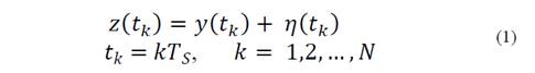
In eq. (1), 𝜂 𝑡 𝑘 are independent additive noise components with 𝐸 ? 𝑡 𝑘 =0, 𝐸 𝜂 2 𝑡 𝑘 = 𝜎 2 and 𝐸 𝜗 is the expected value of 𝜗.
From this signal model, the local approximation theory involves two general problems. The first of these arises when it is necessary to find a polynomial function that can be used to determine the approximate values of a function 𝑦 𝑡 𝑘 . The second problem is related to the use of fitting functions on a given data sequence and determine the best function to represent those data [17,21]. The first problem is associated with the parametric estimation, while the second one is linked with the non-parametric estimation.
2.2. Filtering in the LPA domain
The LPA is a locally adaptive non-parametric technique, which provides estimates of the signal 𝑦 𝑡 ≈𝑦 𝑡 𝑘 defined in eq. (1) from the observations of 𝑧 𝑡 in a pointwise manner and using a polynomial fitting in a sliding window. In this estimation, the error should be as small as possible [22].
In terms of the signal processing, LPA is a flexible tool to design linear transforms with respect to polynomial components of signals. For this reason, to obtain an estimation of 𝑦 𝑡 , the following criterion must be applied on the linear LPA [22,23]:
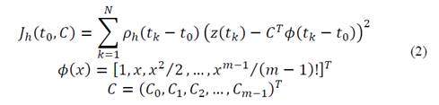
where 𝑡 0 is the point of interest (center), 𝐶 is a vector with the coefficients of the polynomial used during the estimation of 𝑦 𝑡 and 𝑚 is the order of the LPA. The window function 𝜌 ℎ 𝑥 , which formalizes the location of fitting with respect to the center point 𝑥, is a finite support function and must satisfy the conventional properties of the “kernel” used in non-parametric estimation, in particular: 𝜌 𝑥 ≥0,𝜌 0 = max 𝑥 𝜌 𝑥 , 𝜌 𝑥 →0 as 𝑥 →∞ and −∞ ∞ 𝜌 𝑢 𝑑𝑢=1 .
Now, if the function 𝐽 ℎ 𝑡 0 ,𝐶 (eq. (2)) is minimized with respect to 𝐶:

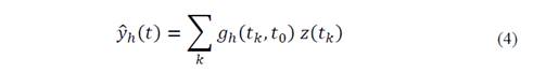
the coefficient 𝐶 0 𝑡 0 ,ℎ = 𝑦 𝑡 0 ,ℎ is an estimate of 𝑦 𝑡 0 with respect to a window function of bandwidth ℎ, while 𝐶 𝑙 𝑡 0 ,ℎ = 𝑦 𝑙 𝑡 0 ,ℎ are related with the estimates of the derivatives 𝑦 𝑙 𝑡 0 with 𝑙=1,2,…,𝑚−1. In this way, the estimates 𝐶 𝑙 𝑡 0 ,ℎ can be represented in the form of a linear transform as follows [15,23]:
where 𝑔 ℎ is the kernel of the estimator defined by [23]:
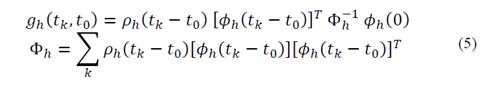
Here, 𝜙 ℎ is a column vector of polynomials of the LPA whose length is equal to 𝑚+1, and Φ ℎ is a symmetric matrix. It is necessary to emphasize that, for a parametric estimation, the order of the polynomial model defines the type of estimation curve (constant, linear, quadratic, etc.) and the coefficients 𝐶 are fixed. On the other hand, in the non-parametric process, the estimate of 𝑦 𝑡 is not a polynomial function and the sliding window estimation makes the coefficients 𝐶 𝑙 𝑡,ℎ different for each point of interest 𝑡 0 .
2.3. Influence of the window function
Mathematically, the window function used in the LPA is expressed by a scale parameter ℎ>0 that determines the window size or bandwidth. For this reason, the window function in eq. (2) and eq. (5) must be replaced by:

Smaller or larger values of ℎ narrow or widen the function 𝜌 ℎ 𝑥 , respectively. The scale factor 1 ℎ in eq. (6) normalizes the window and the property −∞ ∞ 𝜌 𝑥 ℎ ℎ 𝑑𝑥=1 is satisfied. Thus, the polynomial approximation function 𝜙 ℎ also needs to be scaled by the parameter ℎ:

From eq. (4) to eq. (7), it is possible to observe that the length of the window function ℎ controls the smoothness of the estimate 𝑦 ℎ 𝑡 [22,23]. If ℎ is large, the difference between parametric and non-parametric approaches disappears and the estimation function is constant, linear, quadratic, etc., depending on the polynomial degree of the LPA. In this case, the smoothing of random noise in observations is the maximum. On the other hand, when ℎ is relatively small, the estimate 𝑦 ℎ 𝑡 is near (or exactly the same) to 𝑧 𝑡 and there is no smoothing of the data. For intermediate values of the windows size, the resulting curves demonstrate different levels of smoothing.
In eq. (2), if the window is a rectangular function, all observations have equal weights. Nonrectangular window functions such as Gaussian, Hamming, Welch, Hann, etc., usually provide higher weights for observations that are closer to the center point 𝑡 0 . In addition, there are three types of windows (with respect to the center point) that LPA can use: central, right and left windows.
3. Window size selection and the ICI algorithm
3.1. The ICI algorithm and the bandwidth selection
The intersection of confidence intervals (ICI) is a bandwidth selection algorithm that has been proposed and substantiated in several publications [19,22,24-26]. This approach does not require the bias estimation and presents an accuracy approximation better than the quality-of-fit statistics [19]. LPA combined with the ICI algorithm improves the windows size selection process and enables the algorithm to be adaptive. The basic idea of the ICI algorithm uses a finite set of bandwidths 𝐻 expressed by:

Then, for each sample 𝑡 , the LPA-ICI algorithm introduces a sequence of 𝑀 estimates accompanied with the following confidence intervals:

The lower and upper limits of 𝐷 𝑀 𝑡 are defined as:
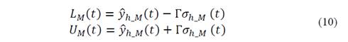
where Γ is the threshold of the confidence interval and the standard deviation of the estimated signal 𝑦 ℎ_𝑀 𝑡 is defined by [15]:

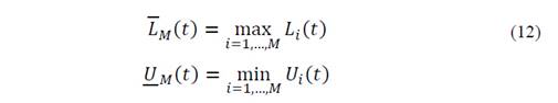
The ICI algorithm tracks the values of the largest lower 𝑈 𝑀 and the smallest upper 𝐿 𝑀 confidence intervals limits:
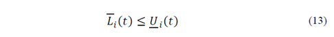
The chosen filter support (bandwidth) ℎ + is the largest 𝑖 support for which the following condition is still satisfied:
It was shown in [15,22] that ℎ + is close to the optimal support ℎ ∗ , which results in the optimal trade-off between bias 𝜔 ℎ 𝑡 and variance 𝜎 2 ℎ_𝑀 𝑡 . Besides, this solution minimizes the MSE [19].
The parameter Γ in eq. (10) plays an important role in the bandwidth selection. A large value of Γ gives ℎ + > ℎ ∗ , producing an over-smoothing in the signal. On the other hand, smaller values of Γ give ℎ + < ℎ ∗ , cause an under smoothing on the signal.
3.2. Threshold parameter Γ
To find the optimal value of the threshold parameter Γ from an theoretical analysis presents great difficulties [15]. For this reason, to compare the performance of the ICI algorithm with respect to Γ, a cross-validation (CV) criteria was selected to assess the statistical prediction. This validation technique has been used to compare the performance of different predictive models [27] and, from the experiments presented in [15,19,28], it can be used as a reasonable and efficient selector of Γ.
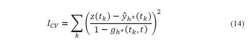
For the linear filter defined in eq. (4), the CV function with an estimator support ℎ + is represented as a weighted sum of the squared residuals [15]:
It is important to mention that the process explained in this section must be repeated for every value of Γ 𝜖 𝑅, 𝑅= Γ 1 , Γ 2 , …, Γ 𝑅 . In addition, the value of the threshold parameter used in the "best" estimation is defined for the following expression:
4. The LPA-ICI denoising method
The main purpose of denoising LEF signatures is to reduce the noise components present in measurements without modifying the most important signal features. Although it is possible to carry out actions to reduce the emissions produced by the measuring system itself, all recorded signals are also distorted by undesired signals from the electromagnetic environment, whose sources cannot be controlled or eliminated.
For these reasons, the method based on LPA combined with the ICI algorithm for noise reduction on LEF signals consists of the following steps:
Set Γ=Γ 𝑅 , for 𝑅= Γ 1 , Γ 2 , …, Γ 𝑅
Determine the sampling time 𝑇 𝑆 from the noisy signal observations 𝑧 𝑡 𝑘 and select a set of samples 𝑡 𝑘 =𝑘 𝑇 𝑆 with 𝑘= 1,2, …, 𝑁
For 𝐻= ℎ 𝑖 , with 𝑖=1,2,…,𝑀, calculate the estimates 𝑦 ℎ 𝑡 and the confidence intervals defined by eq. (12)
Select the largest of those 𝑖 for which 𝐿 𝑀 𝑡 ≤ 𝑈 𝑀 𝑡 gives the bandwidth 𝑖 + =ℎ + . From this result determine the adaptive window size ℎ + 𝑡 and the estimate 𝑦 ℎ + 𝑡 .
Repeat the previous step for all 𝑡 𝑘 and each Γ 𝑅
Find Γ from eq. (15) and select the final estimation of 𝑦 ℎ + 𝑡 𝑘 corresponding to the Γ .
In all cases, the cross-validation presented in eq. (14) and the maximum SNR of the signal (before and after noise reduction) were selected as appropriate indicators for comparing the obtained results. In this paper, the SNR is expressed as the relation between the power of the filtered signal 𝑃 𝑠𝑖𝑔𝑛𝑎𝑙 and the power of noise removed from the measured signal 𝑃 𝑛𝑜𝑖𝑠𝑒 , so:
5. Instrumentation and data
5.1. Typical waveforms of LEF signals
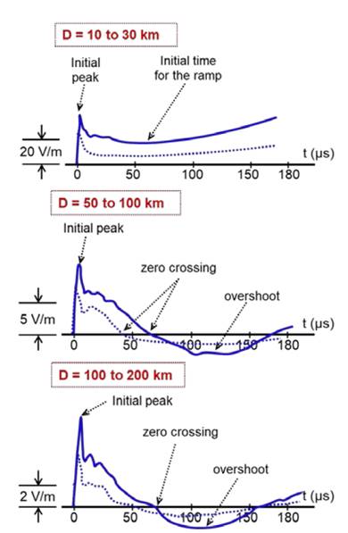
CG lightning flashes are transient discharges of high current that can be generated in the atmosphere by clouds, storms (rain, snow or dust) and volcanic eruptions. A typical CG lightning flash is composed by more than one discharge known as return stroke. These individual discharges have a duration of tens of microseconds and they are usually separated in time from 20 ms to 100 ms [29]. The typical waveforms for the electric fields produced by the first return stroke (FRS) and the subsequent return strokes (SRS) that compose a flash are shown in Fig. 1.
Source: Adapted from [29]
Figure 1 Typical waveforms of the electric field signals produced by CG lightnings with respect to different distance ranges. First return stroke (solid lines), subsequent return stroke (dashed lines).
The most relevant characteristics of these waveforms include: (a) an initial peak with an acute shape (due to a high rate of growth) that decreases approximately with the inverse of the distance; (b) a slow descent ramp after the initial peak that may last more than 100 μs in signals recorded in a nearby range (few tens of kilometers); (c) a zero crossing point that may be several tens of microseconds after the initial peak for the fields registered at distances greater than 50 km; and (d) an opposite-polarity overshoot typical of the electric fields recorded at distances greater than 100 km.
5.2. Measuring system
The typical system to measure LEF was proposed by Cooray and Lundquist in 1982 [30]. In this configuration, an electric field sensor is connected to an electronic circuit for the acquisition of the signal and it is used an equipment to record the data. This arrangement has been used during the last three decades in several regions (Sweden, Germany, Italy, Japan, Sri Lanka, Malaysia, Singapore, USA, Colombia and Brazil), providing valuable information about the behavior and characteristics of lightning flashes [10,31,32].
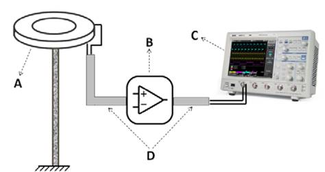
The scheme of the measuring station used in this work to record the LEF signals is shown in Fig. 2, and it is composed by the following parts:
The electric field sensor is a 1.5 meters height parallel flat-plate antenna, which had two circular metallic plates with diameter of 0.45 m supported by insulating elements and 0.03 m air gap between them.
The electronic circuit is based on the buffer-amplifier BUF-602 with 1000 MHz bandwidth and 8 kV/µs slew rate. The decaying time constant of the circuit is 38 ms, which is large enough to record signatures composed by electrostatic (near lightning electric fields) and radiated components (far lightning electric fields).
Two coaxial cables were used to connect the devices. First, a 0.5 m length RG58/U cable was used to connect the antenna to the electronic circuit. Second, a 12 m length RG58/U coaxial cable was used between the electronic circuit and the acquisition equipment.
The acquisition equipment was an 8-bits, digital oscilloscope Agilent DSO6104A with a sampling rate of 10 MSa/s (sampling time of 100 ns).
Source: The authors
Figure 2 Lightning electric field measuring system. (A) parallel-plate antenna, (B) electronic circuit, (C) oscilloscope, (D) coaxial cables.
The arrangement composed by the antenna, the short coaxial cable and the electronic circuit works as a passband filter with a cut-off frequency of 11.8 MHz, which is enough to study lightnings because this range of frequencies covers the bandwidth in which most of the spectrum of the return strokes is found (some hundreds of kHz) [3,12]. A complete description of the measuring system and the electronic circuit, including its calibration process, can be reviewed in [33].
During measurements, the digital oscilloscope was adjusted using a full observation window of 500 ms. This time was selected in order to record a complete CG lightning flash signature that includes the electric field waveforms produced by the first stroke and the subsequent strokes. The vertical trigger level was set at 100 mV to reduce the interference caused by the noise inherent to the measuring system (92 mV average) and to avoid the oscilloscope drive due to pulses caused by intra-cloud lightnings. In order to acquire signals before and after the trigger transient pulse, a 75 ms horizontal pre-trigger was adjusted. In addition, to reduce additional noise that could be produced at the output of the buffer-amplifier, the bandwidth of the oscilloscope was configured in 25 MHz.
Finally, during the pre-processing stage, each return stroke signal (first and subsequents) was extracted from the complete lightning flash signature and it was adjusted for an observation window of 400 µs. Under this condition, using a sampling time of 100 ns, each return stroke signal analyzed in the following sections has 4000 samples.
5.3. Reference signatures
The measurements presented in this section were extracted from the records obtained during August-November 2016. The measuring system was installed in Bogotá, Colombia (4.641° N, 74.091° W) at an altitude of 2550 m above sea level. All the signatures analyzed belong to negative CG lightning flashes. Examples of the recorded events are shown in Fig. 3 and Fig. 4. These signals correspond to normalized signatures of two return strokes (FRS and SRS) and they agree with the waveforms shown in Fig. 1 (distance range between 50 and 200 km). The vertical axis in each plot represents the electric field magnitude in V/m whereas the horizontal axis represents the time in microseconds.
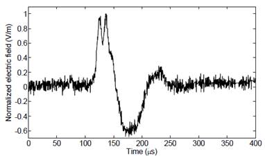
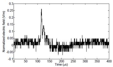
Reviewing Fig. 3 and Fig. 4 it can be seen the presence of noise components that makes it difficult to analyze and characterize the signal features. This is relevant especially in the estimation of temporal lightning parameters, such as: maximum value, signal rise-time (10-90%), zero-crossing time and the maximum electric field derivative, which is an important parameter to estimate the maximum variation of lightning current.
6. Signal processing results
In this section, simulation results of the LPA-ICI denoising method over LEF measurements, the role of the threshold parameter in the ICI algorithm, and the performance of adaptive bandwidths are presented. In addition, the effects of different parameters of the LPA-ICI algorithm are analyzed.
6.1. Simulation parameters
To get a comparative idea about the temporal features and the magnitude of lightning electric field signatures, a set of six return stroke signatures (3 FRS and 3 SRS) were selected. These signals were extracted and normalized from different lightning flashes. In order to analyze the role of the threshold parameter, several values of Γ= 0.01:0.01:4 are defined.
Simulations were performed using a symmetric Gaussian window 𝜌 𝐿 𝑢 = 𝜌 𝐿 −𝑢 . This function was selected because it is well known, from numerical analysis, that symmetric windows result in smaller approximation errors than asymmetric windows [21,34]. The adaptive bandwidths (sample size) for the window function are given by ℎ= {3, 5, 6, 9, 12, 18, 25, 35, 50, 71, 100, 143, 203, 290}.
In order to select an adequate polynomial order for LPA, a linear algorithm was employed by increasing the order of LPA from 𝑚=2 to 𝑚=9 . From simulations, it was observed that polynomial orders less than 𝑚=4 provide results with ripples and remarkable noise components, while high polynomial orders (𝑚≥4) present similar results but increase the computational costs. In this way, a polynomial order of ≥4=5 for the LPA-ICI algorithm was selected for all the cases. Signal processing results were obtained from routines developed in MATLAB® by the authors.
6.2. High SNR environment - first return strokes
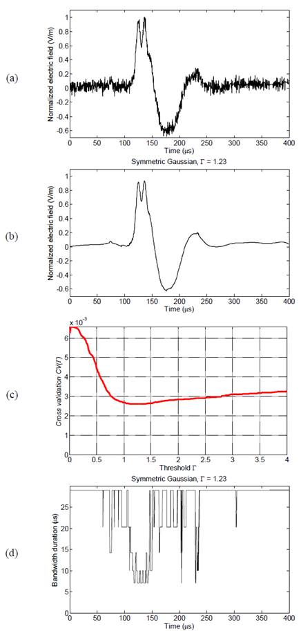
For the example given in Fig. 5(a), the best estimate using a symmetric Gaussian window is presented in Fig. 5(b). In this case, the graphical results illustrate a substantial improvement in the signal features when Γ=1.23. This result is reinforced by the behavior of the threshold parameter with respect to the CV criterion shown in Fig. 5(c).
Source: The authors
Figure 5 Results for FRS signature (Bog3_st1). (a) measured signal; (b) LPA-ICI denoising signal for symmetric Gaussian window with Γ=1.23; (c) CV criterion for LPA-ICI with 𝑚=5; (d) adaptive bandwidth variation.
In addition, the adaptive bandwidths for the adjusted Γ are shown in Fig. 5(d). It can be seen from this curve that at the peak value of 𝑦(𝑡) and at the points where the signal slope changes, the adaptive bandwidths decrease. This means that the LPA-ICI method is sensitive with respect to fast variations of the signal and the symmetrical window presents a good filter response.
6.3. Low SNR environment - subsequent return strokes
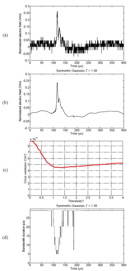
Fig. 6(a) and Fig. 6(b) show the measured signal and the filtered signal of a subsequent return stroke using the LPA-ICI denoising method with polynomial order 𝑚=5. In this case, the denoising result is better because the subsequent stroke signal has a low SNR.
Source: The authors
Figure 6 Results for SRS signature (Bog3_st5). (a) measured signal; (b) LPA-ICI denoising signal for symmetric Gaussian window with Γ=1.38; (c) CV criterion for LPA-ICI with 𝑚=5; (d) adaptive bandwidth variation.
The cross-validation criterion as a function of the threshold parameter is illustrated in Fig. 6 (c) . For the subsequent stroke signal, the minimal value of CV is 4.505× 10 −4 for the adjusted value Γ=1.38. Fig. 6 (d) shows the adaptive varying bandwidths for the symmetric window filter. These bandwidths present faster changes in time, which means that the LPA approximation is enough for denoising the measured signal using the size of windows that are available.
It is important to note that, in this case, the threshold parameter changed from Γ=1.23 (FRS) to Γ=1.38 (SRS), which demonstrates the adaptive response of the ICI algorithm. An advantage of the LPA-ICI denoising method is that the best estimate does not present high noise oscillations and ripples from the measured signal that certainly represent difficulties in the interpretation of lightning parameters.
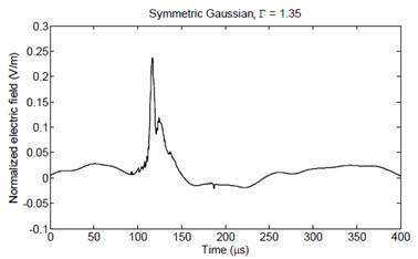
From the best estimate obtained for the SRS signal it was noticed that the adaptive window size, especially for a small value of Γ, could be corrupted by spikes and ripples that erroneously isolate small values of the window sizes. Fig. 7 shows the estimate when the threshold parameter is adjusted from the initial conditions (see section 7.1) to Γ= 0.1:0.25:4.1 .
Source: The authors
Figure 7 LPA-ICI estimates for electric field signature of a subsequent return stroke (Bog3_st5) to Γ= 0.1:0.25:4.1
Note that when the change in the step-size of Γ is made, some ripples in the initial stage of the signal rise and the spikes on the crossing-to-zero region (between 𝑡=1.2× 10 −4 𝑠 and 𝑡=3× 10 −4 𝑠) are slightly reduced. In addition, the threshold parameter of the signal estimate changes from 1.38 to 1.35 with a larger step-size.
7. Discussion
In this work, the parameters selected to analyze LEF are 10-90% signal rise-time (Tr), zero crossing time (ZC) and maximum electric field (Ep). In addition, it is important to know the maximum electric field derivative (𝜕Ep/dt), which is a useful parameter in the estimation of the maximum variation of lightning current. Finally, the SNR improvements after the denoising process are included.
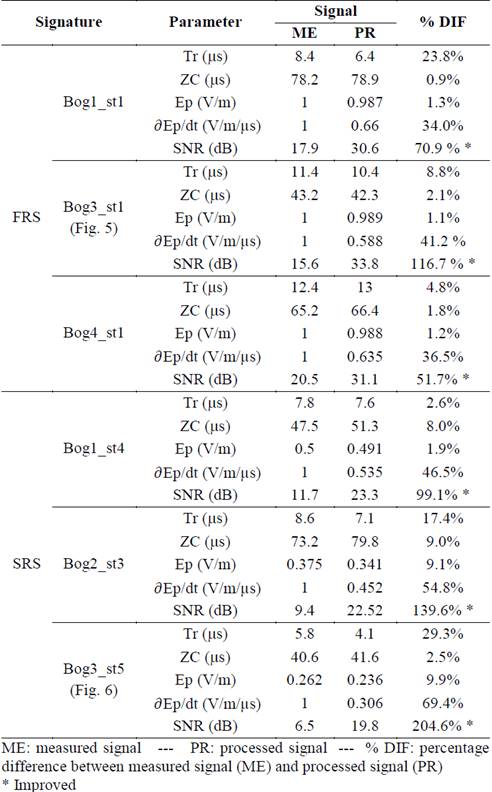
Besides the results obtained from a visual comparison, Table 1 presents the results obtained from characterizing the parameters (Tr, ZC, Ep, 𝜕Ep/dt and SNR) of the signatures before and after noise removal. In addition, the right column in Table 1 (% DIF) presents the percentage difference (for each parameter) between the measured signal and the estimation obtained with the LPA-ICI (processed signal). The maximum values of the electric field and the electric field derivative were normalized taking the maximum of the respective flash as the reference value.
Table 1 Parameters of the LEF signatures before and after the denoising process.
Source: The authors
From the results presented in Table 1, it can be observed that the rise-time presents a difference up to 23.8% and 29.3% in the FRS and SRS cases, respectively. These differences may produce inadequate interpretation of lightning parameters. For the zero-crossing time, the differences were less than 3% for high SNR environments (FRS), while for the low SNR signals (SRS) a maximum difference of about 9% was found (signature Bog2_st3).
On the other hand, the maximum normalized electric field (Ep) shows a variation up to 2% for the FRS signatures, whereas for the SRS cases the variation in this parameter reached 10%. These results indicate that the reduction in the peak value of the signatures depends on the signal noise level. However, it is important to clarify that the removal of noise is directly affected by the selected filtering method.
Regarding the maximum electric field derivative (𝜕Ep/𝜕t), remarkable differences were observed between the measured signatures and the filtered ones. The minimum difference was 34% for Bog1_st1 signature (FRS case) and the maximum difference was 70% for Bog3_st5 signature (SRS case). These results show that the estimation of electric field derivative from the measured signal could be erroneous due to the presence of high frequency noise.
By comparing the SNR of the measured signal with the best result obtained with the LPA-ICI method, it is possible to notice that for the signal Bog3_st1 (shown in Fig. 3 and Fig. 5) the change in SNR ranged from 15.6 dB to 33.8 dB after noise removal. For the signal Bog3_st5 (shown in Fig. 4 and Fig. 6), the SNR exhibits a change from 6.5 dB to 19.8 dB. In general terms, for the whole group of signatures, the improvement in the SNR varied from 51% up to 117% for the FRS cases, while for the SRS cases this parameter was improved between 99% and 205%.
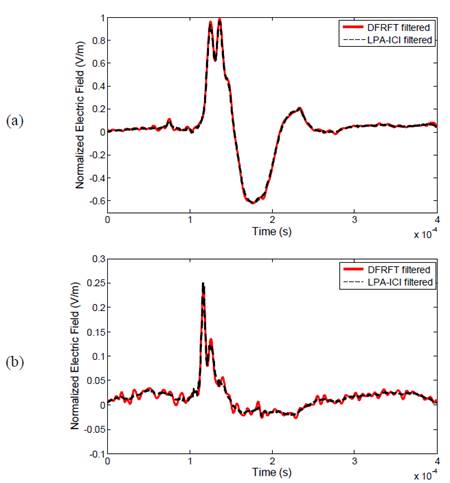
In order to verify the usefulness of LPA-ICI denoising method, a comparison with an alternative method using adaptive filters in the discrete fractional Fourier domain (DFRFd) was conducted. This filtering process is described with detail in [14]. In this work, the adaptive filter in DFRFd is configured with the following parameters: fractional order 𝑎=0.25; normalized leakage LMS adaptive (NL-LMS) algorithm; normalized step-size 𝜇 𝑁𝐿−𝐿𝑀𝑆 =0.95; leakage factor 𝛾=0.997; stabilization factor 𝛽=2∗ 10 −14 ; number of coefficients is 6. Fig. 8 shows the comparison between the signatures filtered with the LPA-ICI method (black dotted line) and using adaptive filters in DFRFd (red continuous line).
Source: The authors
Figure 8 Comparison between LPA-ICI and adaptive filters in DFRFd. (a) FRS signature (Bog3_st1); (b) SRS signature (Bog3_st5)
In this case, it is possible to observed that the LPA-ICI provides similar results than those obtained with the technique based on DFRFT. However, a slight reduction is observed in the peak value of the FRS signature filtered with LPA-ICI algorithm (see Fig. 8a). In addition, adaptive filters in DFRFd introduce oscillations, especially in the SRS signature (see Fig. 8b). These oscillations are typical of Fourier rotated methods, which produce difficulties in the interpretation of some temporal parameters.
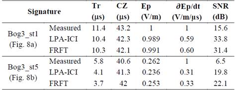
Table 2 Parameters comparison of LEF signatures (Bog3_st1 and Bog3_st5) filtered with LPA-ICI method and adaptive filters in DFRFd
Source: The authors
Table 2 presents the comparison of parameters for signals presented in Fig. 8, which were obtained using both denoising methods. With respect to rise-time, the differences between denoising methods are less than 2% for the FRS signature (shown in Fig. 8a), while for the SRS signature (show in Fig. 8b) the difference reaches 10%. This result in the SRS case is also produced because of the oscillations present in the filtered signal using DFRFT, which do not allow to clearly identify the initial zero-crossing point of the processed signal.
For zero-crossing time and maximum electric field, the differences for both examples were less than 2% and 7%, respectively. The main difference (up to 9%) is presented in the estimation of the maximum value of the electric field derivative for SRS signature (Fig. 8b). This is due to the difference between the maximum value of the filtered signal using LPA-ICI and the output signal obtained with the method based on DFRFT.
8. Conclusions
In this paper, the local polynomial approximation (LPA) combined with the adaptive size window algorithm (ICI) is applied to achieve a successful noise removal process on lightning electric field (LEF) signatures. The advantage of the proposed method compared to other filter methods, as adaptive filters, is that the LPA-ICI does not require a preliminary desired signal that represents the phenomenon.
The proposed method for denoising LEF signals is simple to implement and requires only the calculation of the estimates and their standard deviations for a set of bandwidth values. It is important to note that the LPA-ICI algorithm does not require the estimation of the bias. In addition, the proposed algorithm could be considered an adaptive method because its performance depends on an adequate selection of the window size (bandwidths).
The obtained results show that the LPA-ICI method is efficient to work with non-stationary signals that have jumps, ripples and fast slope changes, such as LEF signatures. In fact, the use of adaptive bandwidths provides better estimates because the most suitable bandwidth controls the smoothness of the filtered signal. In the particular case of LEF signals, the results provided by the LPA-ICI algorithm were found using symmetric Gaussian windows. However, other kinds of symmetric window functions can be tested to analyze the response of the algorithm.
Simulation results, including the effect of window bandwidth ℎ and threshold parameter Γ, were analyzed for both high and low SNR environments. From the tests, it was observed that the change in the step-size of Γ improved the performance of LPA-ICI algorithm. In the low SNR cases, the use of a larger Γ reduces ripples and spikes on several zones of the output signal which are presented when the step-size of Γ is small.
The performance of the proposed method was evaluated in terms of a temporal parameter comparison and the SNR improvement factor for electric field signals produced by first return strokes (FRS) and subsequent return strokes (SRS). Remarkable differences between the measured signal and the filtered signal were found in terms of the rise-time (up to 29.3%) and the maximum electric field derivative (up to 70%). The maximum improvement achieved with respect to SNR was 118% in the FRS cases and 205% in the SRS cases.

