


 English (pdf)
 Article in xml format
 Article references
 Send this article by e-mail
 Cited by SciELO
  Cited by Google
  Similars in
SciELO
Similars in
SciELO  Similars in Google
 Permalink
1. Introduction
The steering system has significant importance in a vehicle dynamic behavior, where its function is to generate angles in the steerable wheels responding to the needs imposed by the driver, so that there is control in the vehicle [1].
The steering mechanism is a main device in the steering system since it allows controlled turn of the steerable wheel, therefore its optimum design is essential. The optimum design of steering mechanisms is not a trivial problem due to its intrinsic complexity and requirement. Generally, a steering mechanism is designed so that axes of steerable wheels and rear wheels axis intercept at the same point, which is called the Ackermann’s condition [2].
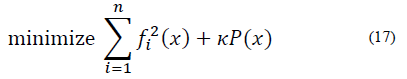
Several works about the steering mechanism synthesis have been published in the last two decades, one of these works is presented by Yao and Angeles, where they propose a method based on a eliminating process to synthesize a four bar mechanism [3], where the goal is to minimize the mean squared of the structural error, so finally the problem is transformed in a system with two unknowns and two equations; and by eliminating one of these unknowns, a polynomial, which roots are local minimums, is obtained. Another work based on minimizing the mean squared of the structural error is shown in [4].
In [5,6] a more complex problem about multilink steering mechanism and McPherson suspension optimization is presented. This problem was boarded using multibody analysis techniques and multi objective optimization. A. Rahmani et al [7], studied the rack and pinion mechanism optimization problem where the goal is to minimize the maximum structural error. Additionally, a sensitivity analysis was made in order to know structural error variability and, in this way, determine that the best option is that mechanism where sensitivity is lower.
A different approach is shown in Collard [8], where links are modeled as deformable elements which deformation energy is minimized in order to find the optimal rigid design. For the model, natural coordinates were also used to simplify and greatly ease the equations that define the mechanism kinematics.
In M. Shariati and M. Norouzi [9], a method for the optimization of a four bar steering mechanism is proposed. This is based on computing the objective function gradient corresponding to the mean squared of the structural error. The objective function is constructed by taking five precision points from which two, correspond to the limit positions, another precision point corresponds to the mechanism straight position, and the remaining precision points correspond to intermediate positions between the limit positions and the straight position.
A. De-Juan et al [10] propose a method of general optimization for steering mechanisms based on the numerical calculation of the Jacobi Method where natural coordinates are used for the kinematics modeling. This is applied to the different steering mechanisms traditionally used. The method’s main advantage is that it can be applied to different steering mechanisms. It can also be used for any other problem of dimensional synthesis of planar mechanisms.
N. Romero [11] proposes a global optimization method using a continuous genetic algorithm, where natural coordinates are used to obtain equations that model the mechanism kinematics. These equations are solved by the Newton-Raphson method [12], where the initial method coordinates are given by the genetic algorithm. The method is applied to all traditional steering mechanisms and to more complicated mechanisms such as the Double-Butterfly steering mechanism.
In this article an optimization global method using a continuous genetic algorithm, is proposed; where the aim is to minimize the structural error of a six-bars steering mechanism. The position kinematic is analytically solved through natural coordinates.
2. Ackermann steering geometry
In Fig. 1, the ideal geometry of the vehicle turning is illustrated where the rotation is around the center I. Mathematically this condition can be written as:
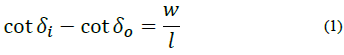
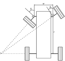
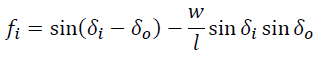
where δi and δ0 are the steering angles of the left and right wheels respectively, 𝑤 is the distance between the pivots of the front wheels, 𝑙 is the distance between the front and rear axle. This eq. (1) is known as the Ackermann steering criterion.
If a vehicle does not fulfill the Ackermann criterion, the front axes intersect at different points with the rear axle, causing sliding on the wheels and therefore, the vehicle is on a general planar motion [13].
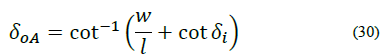
Eq. (1) can also be written as
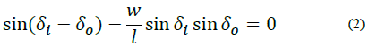
where eq. (2) has a major numerical behavior because the sine function varies between −1 and 1 [3].
3. Kinematic modeling through natural coordinates
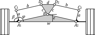
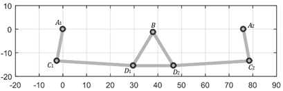
Natural coordinates are mainly cartesian coordinates located in kinematic pairs or interest points [14], this facilitates the modeling of mechanisms since the use of transcendental functions is avoided. Fig. 2 shows the simplicity of modeling using natural coordinates.
Source: The authors.
Figure 2 Modeling of the six-bars steering mechanism using natural coordinates.
To solve the mechanism kinematic position, the parameter φ is chosen as the input, hence the point C1 can be calculated through,
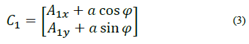
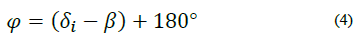
where φ angle and left steering angle are related by:
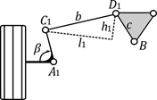
Point D1 is determined using the procedure provided in [15] and [16] , this is described then. From triangle ΔC1BD1 it is possible to determine D1 by means of triangulation, which consists of determining a point given two points and two distances of a triangle. This is possible by writing l1 and h1 (Fig. 3), depending on the triangle distances.
Doing
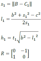
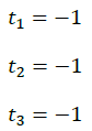
where t1 can take values of 1 or -1, meaning that there are two possible positions of point D1, determined by,
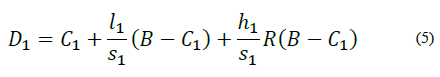
where eq. (5) can be written more compactly as,
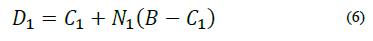
so that
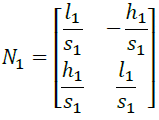
Proceeding in the same way for the triangle ΔD1BD2, it turns out that,

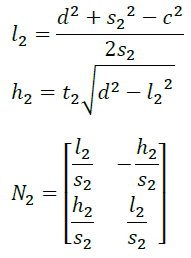
it is obtained

finally, for the triangle ΔD2A2C2 we can write,
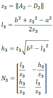
it is obtained
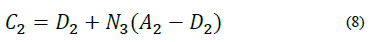
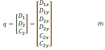
This way, the position kinematics problem is solved, where the natural coordinate vector q is,
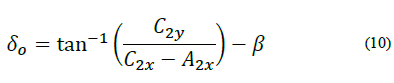
thus, the steering angle of the right wheel is determined as:
The mechanism possible configurations can be represented with the configuration matrix,
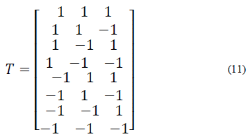
in which each matrix line represents the values of t1, t2, t3. In this case the mechanism has eight different configurations.
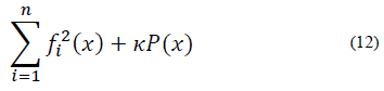
4. Optimization
The objective function is defined as,
where
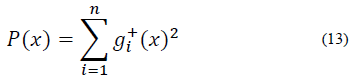
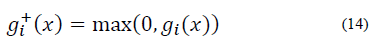
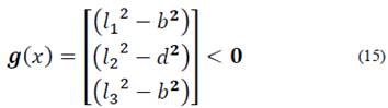
Where gi (x) are the restrictions ensuring that mechanisms have a real configuration. The design variables are contained in the x vector in the following way,

therefore, the optimization problem can be written as:
5. Continuous genetic algorithm
The optimization problem formulation is focused to be solved by using optimization methods where the calculation of derivatives is not necessary. In this case a continuous genetic algorithm is used, which flowchart is shown in Fig. 4. For more detail the reader can see [16].
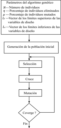
5.1. Selection
Of the NN chromosomes of the population only a percentage η is selected to be crossed. The number of the selected chromosomes to be crossed is determined by,
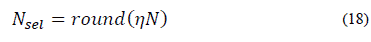
Where round is a default approach to the nearest integer.
5.2. Crossing
The selected chromosomes are randomly crossed as follows,


they are the father i and k respectively. The element α α from PiPj and P k is given by,
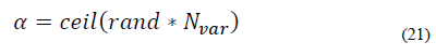
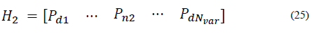
where 𝑐𝑒𝑖𝑙 is an approximation by excess to the nearest integer. The α elements are combined by,


in which τ is a random number between 0 and 1. From this combination result the sons h1 H1 and h2 H2 which are given by:

5.3. Mutation
After having a new population, the percentage µµ of the chromosomes is mutated. The number of mutated elements is given by,
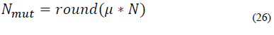
and the chromosome is mutated taking randomly one of its elements and changing it to a new element given by Equation

Where ls and li are the lower and upper bounds respectively.
6. Results
The model proposed for the mechanism optimization of six bars by using natural coordinates was implemented in MATLAB®, for a vehicle with the geometry given in Table 1.

The input parameters of the genetic algorithm used in the optimization are:
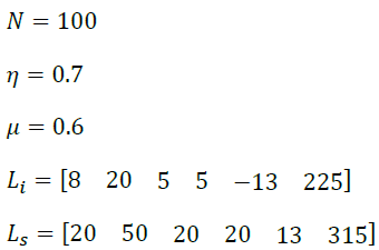
The genetic algorithm was executed for one hour obtaining the optimal dimensions shown in Table 2.

The optimal configuration with the dimensions shown in Table 2, is presented in Fig. 5. Which corresponds to the values of,
The restrictions on the design dimensions of the mechanism are not included in eq. (18), since the limit values of the variables are inputs of the genetic algorithm.
In Fig. 6 the grey line represents the delta optimum Δδ. This is defined by,

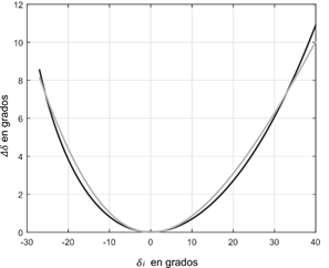
and the black line represents the delta Ackermann ΔδA. This is defined by,

where
This is a way of visualizing how far away the steering mechanism of the Ackermann ideal geometry is, where the difference in the vertical of these two lines, given an angle δi, represents the steering mechanism deviation of the Ackermann geometry.
Fig. 7 shows the structural error of the steering mechanism, defined as,

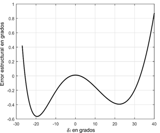
where the maximum error is 0.9 degrees for an angle δ i = 40 °.
6. Conclusions
Use of natural coordinates eases kinematic modeling and formulation of the objective function. In addition, the proposed method can be extended to any steering mechanism where the position kinematics can be resolved analytically or in a closed way.
The genetic algorithm using continuous variables allowed us to deal with the problem, where the main complexity is the high non-linearity of the equations involved in the model.
Although the optimization problem was formulated to be solved without use of derivatives, this does not exclude the possibility of using optimization methods based on the calculation of derivatives.
It should also be noted that the optimization problem was optimized by including integer variables, therefore it can be said that a mixed optimization problem was solved.

