


 English (pdf)
 Article in xml format
 Article references
 Send this article by e-mail
 Cited by SciELO
  Cited by Google
  Similars in
SciELO
Similars in
SciELO  Similars in Google
 Permalink
1. Intoduction
Structural vibrations are undesirable not only for the discomfort caused to users, but also for the fatigue process, which is accelerated by dynamic oscillations. These effects may be detected specifically in structures with low stiffness and low natural frequencies, leading to large displacement amplitudes.
Aiming the reduction of structural vibrations, several techniques were developed to increase structural damping. Among these techniques, the passive control with viscoelastic materials has shown reasonable efficiency. In order to effectively reduce structural vibrations using this technique, it is important to understand the dynamic behaviors of the structure and of the viscoelastic material (VEM).
Due to the mechanical properties frequency dependence on VEM, time domain based models are not so numerous as frequency domain methods. In spite of that, because of the facilities that time domain methods may directly provide, such as the maximum displacement range in a structural model analysis, many researchers have been developing numerical methods to simulate the VEM dynamical response in the time domain. The most successful models are the ones that introduce extra dissipation coordinates or internal variables in a Finite Element, due to its simplicity and capability to virtually model any complex geometry. This kind of methodology has been applied in several situations such as the ones presented by Friswell et. al [1], Roy et. al [2], Wang et. al [3] and Wang et. al [4]. Among the dissipation coordinates based methods it is possible to observe that Golla-Hughes-McTavish (GHM) method [5,6] and Anelastic Displacement Field (ADF) method [7-11] are frequently chosen in order to simulate the dynamic response of VEM.
Within this context, this paper will discuss the computational modeling of VEM and their use for reducing vibrations in structures, working as a passive control mechanism in sandwich layers. Computational viscoelastic sandwich models, based on GHM and ADF methods, are analyzed and their results are compared with theirs theoretical counterparts. Finally, an actual structure is used to evaluate the facilities and difficulties of each applied technique.
2. Viscoelastic materials modelling
2.1. The GHM model
The stress-strain relation for a single degree of freedom system on Laplace’s domain, as mentioned by reference [5], may be written as:
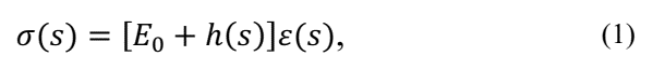
where s is the Laplace operator, σ
σ(s) and
 are, respectively, the stress and strain on Laplace’s domain, E
0 is the elastic fraction of complex modulus and h(s) is the relaxation function.
are, respectively, the stress and strain on Laplace’s domain, E
0 is the elastic fraction of complex modulus and h(s) is the relaxation function.
Function h(s) can be written using Biot’s [12] series, with two terms as:
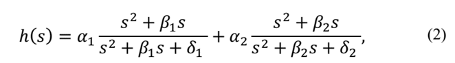
where
 are materials constants and
 .
.
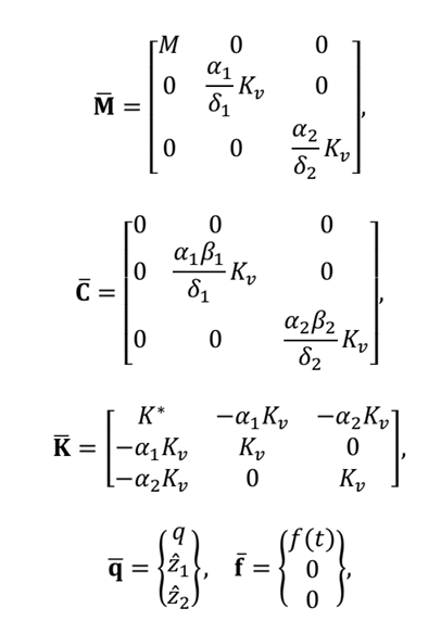
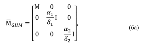
The GHM model is developed starting from the equation of motion in the Laplace domain:
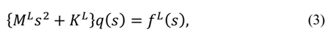
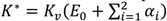
where, M L , K L and f L are respectively the mass, stiffness and external loading in the Laplace domain, being:
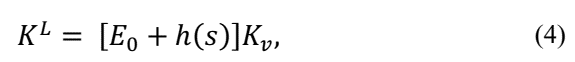
and K v is the rigidity associated with geometrical characteristics of the model.
The GHM model defines the equation of motion in the time domain as:
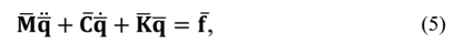
where:
ẑ
i
is the auxiliary variable introduced into the problem, called dissipation variable, and
 .
.
Generalizing eq. (5) for n degrees of freedom, then this equation may be written as in eq. (6):

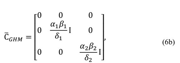
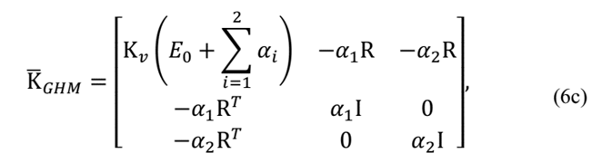
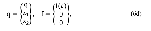
and where:
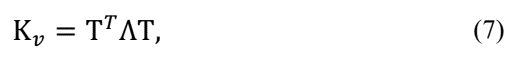
being Λ a diagonal matrix consisting of the non-zero eigen-values of the stiffness matrix normalized with respect to the elastic modulus, E; Tthe matrix of vectors corresponding to the non-zero eigen-values of the matrix 1/E
K
elastic
, where K
elastic
the elastic Finite Element stiffness matrix is; R=T Λ
1/2 and

As shown in eq. (2) and (6) the number of dissipative degrees of freedom associated with viscoelastic elements depends on the number of terms used in relaxation function and the number of rigid body motions [13]. It should be noted that the greater the number of terms used to write the relaxation function the more accurate the modelling.
Using eq. (6) and (7), it is possible to determine stiffness, mass and damping matrices, for any kind of Finite Element.
2.2. The ADF model
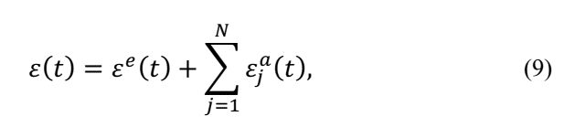
Lesieutre [9] establishes that the displacement field can be written as:
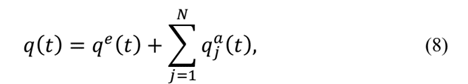
where q e(t) is the elastic displacement field and q a j (t) is the j-th anelastic displacement field are then the strain field is defined as:
The ADF model defines the equation of motion in the time domain as

where σ(t) the stress in material is. Considering eq. (9) one can obtain:
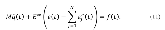
where E ∞ the elastic modulus at high frequency is. Defining the anelastic stress as a “thermodynamic force” that carry the anelastic deformations to an equilibrium point Lesieutre [9] defines:
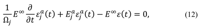
where E a j the j-th anelastic modulus is and Ω j it is a material parameter. Applying the Finite Element Method on eq.(11) and (12) and considering just two terms on eq. (8) one can write:

where

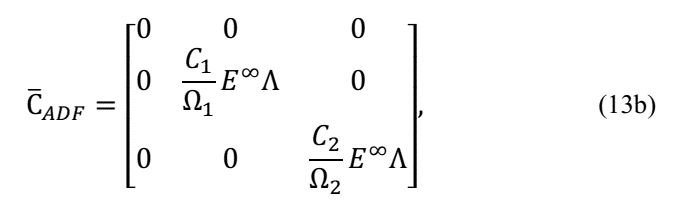
C j it is a material parameter and, as in GHM Model: K v =T T ΛT.
As shown in eq. (8) and (13) the same observations about the number of dissipative degrees of freedom associated with viscoelastic elements can be made as the ones made for GHM model.
3. Evaluation of VEM models
3.1. The GHM model
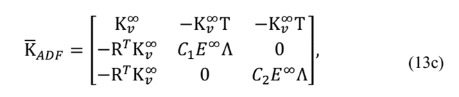
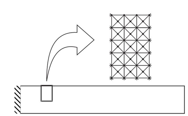
The validation test applied to both methods consists of evaluating the dynamic behavior of a viscoelastic cantilever beam. The beam has rectangular cross-section and 1000mm length; the cross-section has 300mm height and 150mm width as shown in Fig. 1.
The numerical simulations ware performed using triangular element (constant strain triangular elements - CST) meshes to discretize the domain of the structures. In order to obtain the suitable refined mesh a convergence analysis was performed until no significant difference was observed for two levels of refinement. Once defined the configuration of the mesh for each tested beam model, this mesh was used for the both formulations - GHM and ADF. The refined mesh has 602,302 physical dof and 1,800,000 dissipative dof, 2,402,302 dof total. A schema of the used mesh is presented in Fig. 2. The viscoelastic triangular elements matrices were obtained with eq. (6), for GHM Model, and eq. (14), for ADF Model.
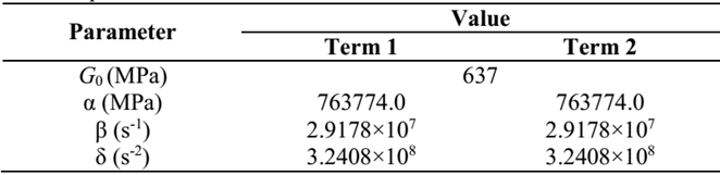
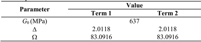
In order to better evaluate the accuracy of the analyzed methods, two VEM were used for the validation. For GHM’s and ADF’s tests, materials 1 and 2, respectively, were applied. Tables 1 and 2 present the parameters of these materials used in eq. (6) and (13) to obtain the VEM cantilever models. This strategy was adopted due to the differences in the expressions for the complex modulus for the two formulations.
GHM and ADF formulations allow time domain equations for VEM. However, using their respective frequency domain equations, it is possible to apply classical discrete solutions to compare and evaluate the quality of GHM and ADF results, as is explained below.
Starting from the dynamic equilibrium equations, using the complex excitation one has the classical discrete equation:

where M is the structure mass matrix;
 is the frequency dependent stiffness matrix on the structure;
 is the harmonic excitation vector having ω as the excitation frequency and
 . It can be noticed that, if the mechanical properties of the structure are not frequency dependent,
 , which is not the case of VEM.
Using GHM or ADF, eq. (14) may be rewritten as:
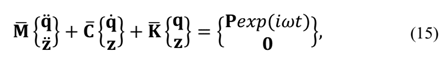
where,
 and
and
 the mass, stiffness and damping matrices for GHM or ADF are respectively. It is important to notice that the stiffness matrixes in the GHM or ADF formulations are not frequency dependent.
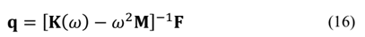
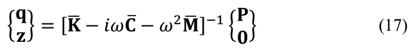
The frequency domain displacements, q, may be obtained by solving eq. (15) and (16), resulting in eq. (17) and (18), respectively:
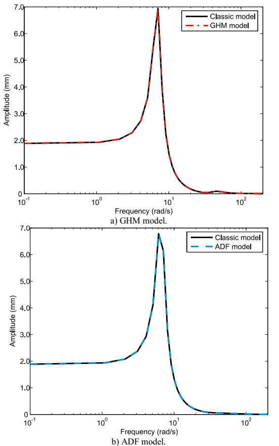
By solving eq. (16) and (17) for the two beam models, the graphs in Fig. 3 may be achieved. It is possible to observe that, for all tested beam models, ADF and GHM formulations allow identical results when compared to the respective classical responses, supporting the accuracy of applied methods. Fig. 3.a and 3.b were achieved observing the vertical nodal displacements at the free end of the beam models, with only one nodal harmonic transversal load also at the free end. As can be seen in this figure both models produce the same response on the frequency domain as the Classic model.
3.2. Time evaluation of numerical methods
Another parameter to compare both methods is the time taken to assemble the models global matrixes. Both methods ware implemented virtually with the same code in MATLAB where each program uses global sparse matrixes; Assembles the global matrixes element-per-element; and for each element, an eigenvalue problem is solved.
In an Intel Core 2 Duo computer with 2.1GHz clock and 2.00Gb RAM the VEM cantilever beam models were evaluated 20 times, running under a Windows Vista operational system, and the total time taken to assemble the global matrixes and impose the boundary conditions were registered. The time taken to solve the time problem and to solve the dynamical system were disregarded.
With these registered times the histograms on Fig. 4 were able to build. For the GHM model the mean time is 8.97h with standard deviation 1.83 and coefficient of variation 0.24; and for the ADF model the mean is 8.00h with the standard deviation 0.79 and coefficient of variation 0.10.
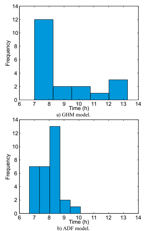
One can notice that the mean times of both models are close but the ADF model coefficient of variation is about half of the GHM model.
4. Experimental evaluation of VEM models
4.1. Experimental program
In order to evaluate the viscoelastic models, an experimental program was developed. In these laboratory studies, a set of three kinds of sandwich beams was tested. The beams were divided into three groups in accordance with its layer configuration:
a) VS1 beam, with two elastic layers (base beam and clamped restraining layer) and one viscoelastic layer;
b) VS1c beam, with two elastic layers (base beam and free restraining layer) and one viscoelastic layer and;
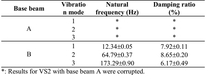
c) VS2 beam, with three elastic layers (one base beam and two clamped restraining layer).
The layer configurations of each sandwich beam group can be seen at Fig. 5.
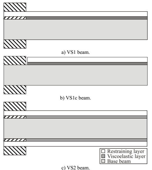
All beams have rectangular cross section and 1140 mm length, working as the elastic base structure with 16,1mm height; viscoelastic layers with 2,0mm height; and elastic constraining layers with 3,17mm height.
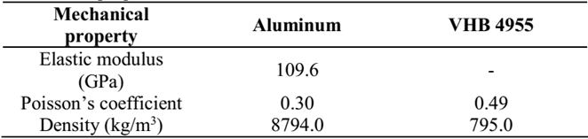
The elastic material was aluminum and the viscoelastic material used was VHB 4955 [14], their mechanical properties are listed in Table 3.
Two geometrically identical based structures (Base beam A and B) were used for each group of beams. This strategy was applied in order to evaluate the experimental result dispersion. For exact identical Base beams, one should have identical results.
The beams were excited under the action of a hammer impact at 15 cm from cantilever and at the same section the transversal displacements were measured with LVDT sensors, which could register displacements without touching the structure.
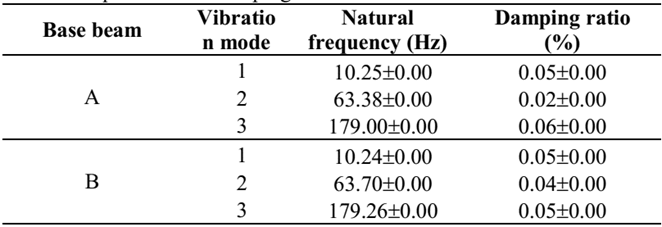
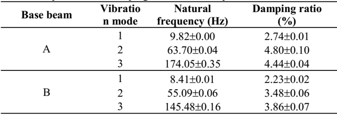
For the two base beams (A and B) used as base structures, without damping treatment, the natural frequencies and their damping rates are listed in Table 4, respectively.
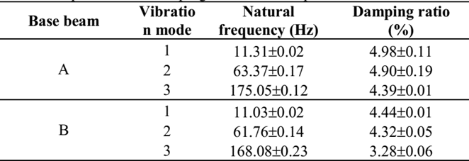
For the three specimens with damping treatment, their natural frequencies and damping rates are listed in Tables 5-7, respectively.
4.2. Models parameters
There are several methodologies for characterizing the Complex Modulus of viscoelastic materials: ASTM Standard Method [15], Direct Method [16] and Indirect Method [17]. These methods basically register, at a given temperature, the temporal responses, when a specimen is submitted into shear or axial deformation [18].
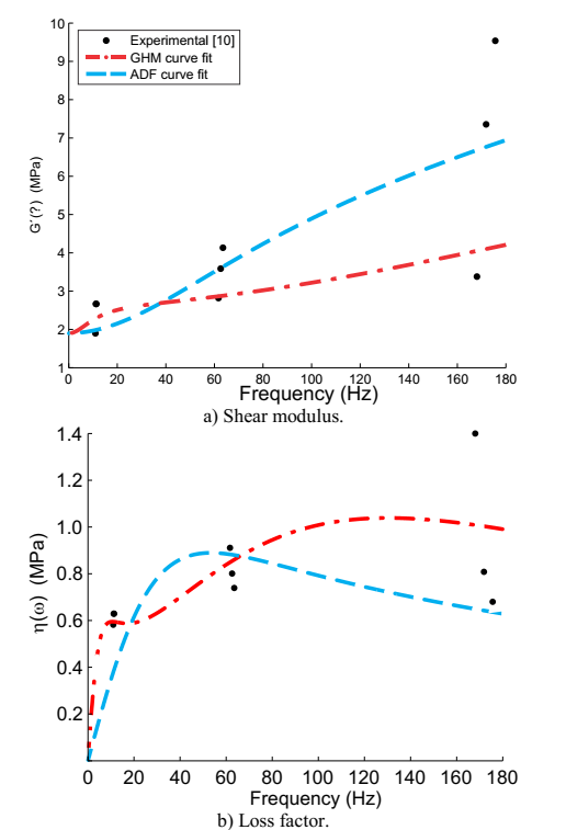
After the values of Complex Modulus are experimentally determined, one can adjust the curves of the real part of the Complex Modulus and the loss factor for the points obtained experimentally. In the case of the formulation GHM, they are given, in terms of shear modulus, by:
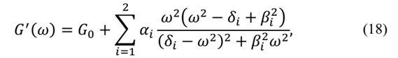
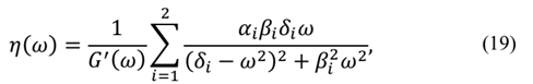
and in the case of the ADF formulation these equations are:
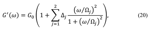
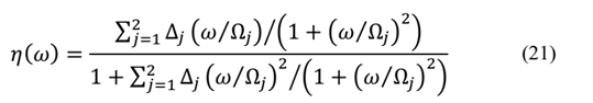
these functions are used to determine the GHM and ADF materials parameters.
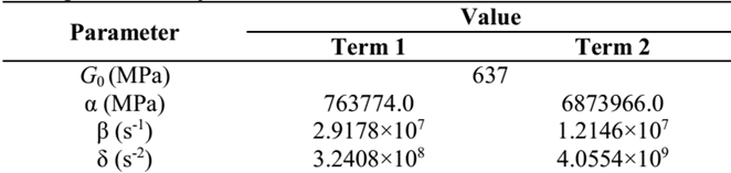
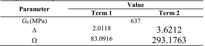
In this paper, the Direct Method was applied for frequencies between 0 and 200 Hz. Using data from the experiments, the materials parameters could be determined using the Nonlinear Least Squares Method [19, 20]. These fitted values are shown in Table 8, for the GHM Model, and Table 9, for the ADF Model. Fig. 6 shows two graphics comparing the experimental values and the adjusted curves of G′(ω) and η(ω) for both models.
4.3. Numerical evaluation
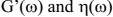
The viscoelastic triangular elements matrices were obtained with eq. (6), for GHM Model, and eq. (13), for ADF Model. The discretized beams were excited using an impact model, shown in Fig. 7, at 15 cm from cantilever and, at the same point, the transversal displacement along the time was observed.
The same elastic layer mechanical properties and viscoelastic layers ware considered in Table 3 in addition to the GHM and ADF parameters previously listed in this section.
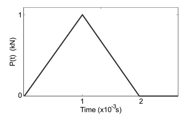
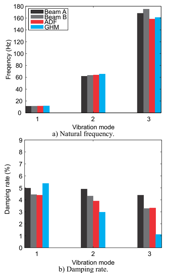
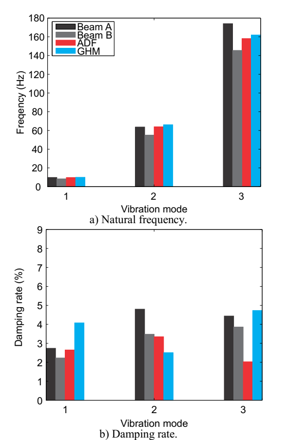
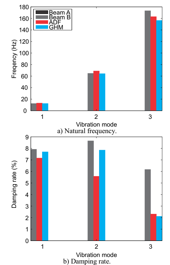
With the models, meshes and mechanical properties described, the time response of beams could be obtained. In order to obtain the natural frequencies and damping rates it was constructed the spectral response; The first three natural frequencies were identified; The time response signal was filtered around these frequencies and; The damping rates were obtained. The relationship between the numerical and experimental data could be seen on Fig. 8 through Fig. 10.
Source: The authors.
Figure 8 Relationship between the numerical and experimental data for VS1 beam.
Source: The authors.
Figure 9 Relationship between the numerical and experimental data for VS1c beam.
5. Conclusions
This study evaluated the GHM and ADF methods on computational modeling of viscoelastic materials acting as structural vibration dampers. These models were implemented in a finite element code and were observed that both produce the same response on frequency domain and results nearly to those obtained in the experimental program.
Analyzing the obtained responses for the experimentally studied beams, one can observe that natural frequencies obtained with both presented models, in general, have good agreement with the experimental counterpart for the first three modes.
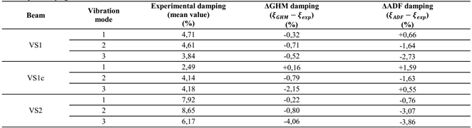
In Table 10, are shown the absolute differences, in terms of damping rates, between the experimental and numerical results. As could be seen, in general, the GHM model presents a better agreement than the ADF model. It could be stated that GHM model evaluated damping rates with differences, in terms of percentual points, between -0,32 and +0,16 for first vibration mode; between -0,80 and -0,71 for second mode and; between -4,06 and -0,52 percentual points for third mode. For the ADF model these differences are between -0,76 and +1,59 for first vibration mode; between -3,07 and -1,64 for second mode and; between -3,86 and +0,55 for third mode.
It is important to emphasize that material functions with two terms in both models were adopted and it is possible to see in Fig. 2 that the curve fit for ADF model was better than that obtained with the GHM model. It can also be highlighted that the Nonlinear Least Squares Method is an iterative curve fit method and a higher number of attempts was needed to get a good fit with the GHM model than with the ADF model.
By analyzing the obtained responses for the cantilever beams, one can observe that despite the good correlation between the fitted curves and the experimental data, the damping factor obtained through the numerical models were, in general, underestimated for both models, while the good agreement of natural frequencies obtained with the models and the experimental values. Obviously these differences cannot be attributed only to curve fitting. Other factors such as: the methodology used on modal identification (in numerical evaluation the exponential decrement methodology was adopted and in laboratory tests the half power method was adopted); 2) Dispersion of experimental results; 3) The Finite Element discretization, also play a significant influence on numerical results.
It could be also observed that the adopted damping treatment, in both cases, considerably increased the damping rates of the structures when compared with the elastic structure without damping treatment. This structural behavior allows the conclusion that viscoelastic materials may be used to reduce vibration oscillations.
Despite the fact that both models provided results close to experimental data and in favor of safety, the curve fit and the results obtained with the ADF model were better than the ones obtained with the GHM model. It seems that considering the formulations presented here the ADF model is more suitable to model viscoelastic materials than the GHM one.


