


 Inglês (pdf)
 Artigo em XML
 Referências do artigo
 Enviar este artigo por email
 Citado por SciELO
  Citado por Google
  Similares em
SciELO
Similares em
SciELO  Similares em Google
 Permalink
1. Introduction
Currently, when a phenomenon is studied, measurements of different variables are taken over many observation units, generating large volumes of data. Multivariate statistical methods are appropriate in these situations because they consider the existing relationships between variables [2]. In some circumstances, these variables are qualitative, and a method that is frequently used for extracting information from these types of variables is the multiple correspondence analysis (MCA) technique. However, this method only works with complete information, that is, it does not allow the presence of missing data.
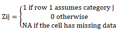
MCA is widely used in the analysis of surveys with questions that must be answered with only one of several options [13]. The answers to these types of questions generate qualitative variables (nominal or ordinal), each of which are associated with splitting the individuals (disjoint groups of individuals). When a question is not answered, nonresponse (NR) or missing (NA) data are generated.
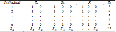
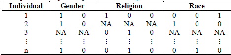
A table, which is the object of MCA analysis, has the statistical units in rows and the qualitative variables in columns. Each statistical unit, called an “individual”, assumes only one category of each variable. A table that is analyzed with MCA has as many columns as variables, which indicate the categories assumed by the individuals. Because this table does not have a numerical meaning, it is transformed into a table of individuals by categories, where each qualitative variable generates as many columns as it has categories. This table is called a complete disjunctive table (CDT) because for each row within the columns of each variable there is only a single value of one, which indicates the category assumed, and the remaining columns are zero (see Table 1). The theoretical approach of the MCA starts from the CDT.
The MCA is the correspondence analysis (CA) of the CDT, which has very unique properties that are lost in the presence of missing data. Van der Heijden and Escofier [23] compare several methods including missing passive, missing passive modified margin, missing single, and missing multiple.
The missing passive method is equivalent to performing a correspondence analysis of the incomplete disjunctive table (IDT), which is called that because in the case of a nonresponse for a variable, the row has zeros in all the columns of the categories of that variable [7,14]. The missing passive modified margin method [7] is proposed to recover most of the MCA properties.
The missing single method, one of the most used, consists of creating a category for each variable with missing data. This option is usually managed by the analyst, who recodes the data prior to introducing them into an MCA program [23].
Currently, there are other authors working with missing data using the nonlinear estimation by iterative partial least squares (NIPALS) algorithm in multivariate analysis [1,18,19,22], and others working on the data imputation approach with the expectation maximation (EM) algorithm [3,11,12]. It is not exactly known which approach generates better results; however, works have been found that compare them to principal component analysis (PCA) [24].
In the case of MCA with missing data, authors Josse et al. [12] have worked with the EM algorithm approach, experiencing difficulties in the imputation process of the complete disjunctive table; it assigns one to the higher-frequency categories and presents some convergence problems. However, there are no known works or ideas that attempt to work with MCA under NIPALS. For this reason, this research proposal will generate more knowledge on how to process missing data with MCA.
In this work, it is proposed to use the NIPALS algorithm by Wold et al. [25] to perform MCA with the available data, that is, without the imputation of the missing data. The proposed method, called multiple correspondence analysis under the available data principle (MCAadp), evaluates the influence of this type of data on the factorial axes, the descriptive power (percentage of applied variance), and the inertia generated in each component, among others. This procedure can be seen in more detail in [15].
The MCAadp method is illustrated with the DogBreeds database of the FactoClass library of the R software [4,17]. It begins with the complete database and missing data are randomly generated in different percentages, i.e., 5%, 10% up to 50%.
The following contains a summary of the MCA, NIPALS algorithm, iterative MCA (iMCA), and proposed MCAadp methods.
2. Methodologies
In this section, the MCA method and the NIPALS algorithm are theoretically presented. The NIPALS algorithm is used to work in the presence of missing data, using the available data principle. In addition, each method, their optimization processes, the matrix to diagonalize, the concept of inertia, the eigenvalues, eigenvectors, and additional concepts that are relevant to the multivariate analysis are explained. This section also refers to the existing relationships between methods, especially that the MCA is a PCA of a matrix transformed into weighed profiles [13,21]. In the last subsection of this section, the method for the imputation of the data based on the EM algorithm for the MCA is explained. The MCA is presented below.
2.1. Multiple Correspondence Analysis (MCA)
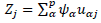
The principles of this method can be credited to Guttman [8], Burt [5], and Hayashi [9]. MCA is used in the analysis of tables of individuals described by qualitative variables and to study the associations between different categories of variables being studied [13,16]. MCA is a generalization of CA, defined as an CA of the complete disjunctive table Z, where the number one is assigned to the category assumed by the individual, and zero to the category that was not selected, as observed in Table 1.
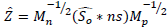
F is obtained from matrix Z, with the following general term:
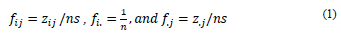
where s is the number of qualitative variables and n is the number of individuals.
2.1.1. Maximization and matrix to diagonalize
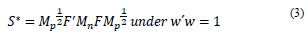
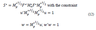
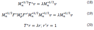
The MCA geometric goal is to find a new system of orthogonal axes 𝑢α, where the inertia 𝐼𝐼 of the cloud of individuals is projected such that the first axes concentrate most of the inertia in decrescent order. In this manner, the factorial coordinates Ψ α are obtained; they are the projection of the individuals over the space generated by u α , where α =1,2,…,𝑝−𝑠. It is important to mention that the diagonal matrices 𝑀𝑛=[⋱1𝑓𝑖.⋱] and 𝑀𝑝=[⋱1𝑓.𝑗⋱] correspond to the metrics associated with the individuals and the categories. The inertia associated with the space of individuals is I= Ψ′𝑀𝑛−1 Ψ, with Ψ=𝑀𝑛𝐹𝑀𝑃𝑢, that is, 𝐼𝐼=𝑢′𝑀𝑝𝐹′𝑀𝑛𝐹𝑀𝑝𝑢, which is the amount to maximize under the constraint 𝑢′𝑀𝑝𝑢=1.
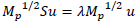
The Lagrangian solution leads to the system of eigenvalues and eigenvectors Su = λu, with S = F´M n FM p and u´M p S u = I = λ, which correspond to the highest eigenvalue.
Matrix S is not necessarily symmetric; therefore, it does not guarantee that the eigenvectors are orthonormal. Observe from the previous system that
 , as follows:
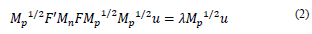
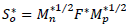
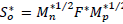
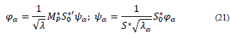
Instead of diagonalizing S, matrix S * is diagonalized, as follows:
The eigenvectors
 are orthogonal and are associated with the λ- eigenvalues of S
*. Note the following:
are orthogonal and are associated with the λ- eigenvalues of S
*. Note the following:
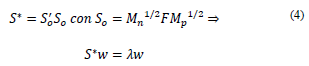
In this way, the relationship MCA has with PCA is observed, where MCA is a PCA of the symmetric matrix S * [13,21]. Similarly, matrix T * = S 0 S’0 is diagonalized in space R n.
This scheme is very important because it is also followed for the solution with missing data, using the available data principle.
2.1.2. Total inertia of the cloud of categories
The inertia of the cloud of categories p is as follows:
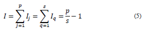
where I j is the inertia contribution of a category and I q is the inertia associated with a variable, i.e., the inertia of the subcloud of its categories.
2.1.2.1. Inertia contribution of a category
To calculate the inertia contribution associated with a category j, its weight is considered, i.e., the marginal column f ,j = z ,j/ns and its distance to the center of gravity. In this way, the inertia by modality I j is as follows:
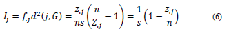
The inertia contribution of a category is higher if there is low frequency in the data set.
2.1.2.2. Inertia by variable
The inertia due to a variable (subtable) q is an increasing function of its number of categories p q . The inertia by variable I q is calculated as follows:
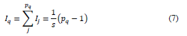
In the presentation of the MCAadp method, how to calculate the inertia expressions in the presence of missing data will be emphasized.
2.2. Nonlinear Estimation by Iterative Partial Least Square (NIPALS)
The NIPALS was proposed by Wold and is the basis of the partial least squares (PLS) regression [20]. It essentially performs a decomposition of the data matrix into singular values by iterative sequences of orthogonal projections (geometric concept of regression) obtained as point products. When the database is complete, there is an equivalence with the PCA results, and it can also work with missing data and obtain estimations from the reconstituted data matrix.
For the data matrix Z
n,p
of range a, whose columns Z1,…,Zp are assumed to be centered or standardized, the decomposition derived from the PCA allows the reconstitution by
 , where Ψ
α
is the α-th principal component and u
α
is the eigenvector associated with axis α [1]. Then, it is possible to make the reconstitution by individuals or variables, where
, where Ψ
α
is the α-th principal component and u
α
is the eigenvector associated with axis α [1]. Then, it is possible to make the reconstitution by individuals or variables, where
 for j = 1, … , p and
 .
.
The algorithm begins by taking the first column of Z0 as the first principal component Ψ 1 . Then, a series of deflated tables will be constructed, called Zα = Z0 - Ψ α u α , which allow the cycle to restart and the remaining components (orthogonal) Ψ 2 , .., Ψ p , and their respective eigenvectors u1, … , up to be obtained.
Shown in the following subsections is the pseudocode of the algorithm when the data matrix is complete. As observed in stage 2.2.1, u αj represents, prior to the normalization, the coefficient (slope) of the regression of Zα−1,j over component Ψ α .
2.2.1. NIPALS algorithm pseudocode
Stage 1: Z0 =Zh
Stage 2: α =1,2, … , p
Stage 2.1: Ψα= 1st first column of Zα-1
Stage 2.2: Repeat until convergence of uα
Stage 2.2.1:

Stage 2.2.2: Normalize Uα to 1
Stage 2.2.3:

Stage 2.3: Zα = Zα-1 - Ψα uα’ (ensures orthogonality)
Next, α
2.2.2. Available data principle
This principle refers to some operations between vectors, omitting the missing data and working with the available matched points; that is, if there are two vectors with NA, {x,y} can be found using the available data principle [15].
Then:

Note that the same result is obtained if the NA are replaced with zeros.
2.2.3. NIPALS missing data algorithm pseudocode
Stage 1: Z0 = Zh
Stage 2: α = 1,2, …, α
Stage 2.1: Ψα = 1st first column of Zα-1
Stage 2.2: Repeat until convergence of uα
Stage 2.2.1: For j=1,2,...,p
Stage 2.2.2: Normalize 𝑢 𝛼 to 1
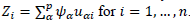
Stage 2.2.3: For i = 1,2,...,n
Stage 2.3: Zα = Zα-1 - Ψαu´α
The main characteristic of NIPALS is that it works with a series of point products as a sum of products of the matched elements. This allows it to work with missing data by adding the available data in each operation. Geometrically, the procedure considers the omitted elements falling over the regression straight line; they are not leverage points [20].
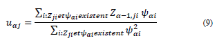
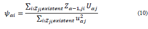
The pseudocode of the NIPALS algorithm with missing data contains stages 2.2.1 and 2.2.3, where the slopes of the lines of the least squares from the origin of the point cloud over the available data are calculated. uαj and Ψαi must capture, in their positions j and i, the missing data characteristic given by Zij [1].
2.3. Iterative MCA for missing data (MCA-EM)
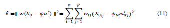
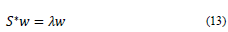
The iterative MCA via EM (iMCA or EM-MCA) was proposed by Josse [11]. This method is based on the EM-PCA, where the missing data are estimated by average values, and then the distances between the original data 𝑆 𝑜 and the estimated data Ψu are minimized, such that the iMCA uses the following loss function:
Where
 , is the complete disjunctive table, Ψn,q is the factorial coordinates, u p.q is the eigenvector in Rp, α = 1,2,…,q (q<p-s) , and w is an indicator variable (0 = NA; 1 = observed value). As in EM-PCA, this method minimizes the loss function associated with the complete data [12]. Presented in the following subsection is the pseudocode associated with the iMCA method.
2.3.1. iMCA algorithm pseudocode
1. Initiation L = 0: Z0
The missing data are replaced by the proportion of ones in the complete disjunctive table Zij. The replacement of the missing data must add one per variable, which makes the marginal per row equal to s, as in the complete data.

2. Step L
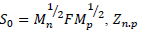
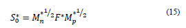
2.1 Perform a singular decomposition of matrix 𝑆0=𝑀n1/2𝐹𝑀1/2 (Ψ and 𝑢 are obtained here).
2.2 Perform the reconstitution of matrix
 , using the q dimensions (q < p -s) found by generalized cross-validation.
2.3 Perform the reconstitution of the complete disjunctive table
 . Here, the missing values are imputed with the reconstitution and the observed values of Z are the same.
Steps 2.1, 2.2, and 2.3 are repeated until convergence, where one is assigned to the highest-frequency category in
 and zero is assigned to the remaining categories.
3. MCAadp: Multiple Correspondence Analysis under the available data principle
The MCAadp method in the presence of missing data is presented in this section. Methods to obtain the eigenvalues and eigenvectors in spaces Rn and Rp are shown. From these results, the transition relations are considered for finding the components in each space. In addition, the expressions of Total Inertia, Inertia by question, and Inertia by category are presented. With this method, the proposal by Wold [25] and the multiple correspondence analysis are adapted to work with missing data [15]. The MCAadp method is presented below.
3.1. Presentation of the MCAadp Method
To perform MCAadp, first, a disjunctive table with missing data Z*n.p is constructed, as presented in Table 2.
Second, the relative frequency matrix
 is calculated. In this process, it is important to consider that when building,
 is performed, where

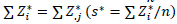 ; it is obtained by adding by rows or columns to obtain the corresponding marginals, this time with the available data.
Note that if the NA are replaced with zeros, the same result is obtained in the marginals and in the sum of the table.
3.2. MCAadp in space Rp
Based on the relationship between MCA and PCA, the matrix to diagonalize is as follows:
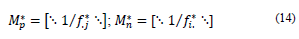
In the diagonalization process of matrix S* is the following system of eigenvalues and eigenvectors:
Then, S* contains the submatrices
 , such that
 . It is important to mention that Mn* and Mp* are obtained with the available data and correspond to the metric matrices for the row and columns, respectively. These are diagonal matrices that contain said weights in their diagonal. In detail, the matrices have the following structure:
Thus, matrix
 is obtained, which does not contain missing data, since the available data principle is considered when performing the point products.
Finally, for matrix S0*, a decomposition into singular values is executed iteratively, as performed by the NIPALS algorithm.
3.3. MCAadp pseudocode
The disjunctive table is constructed with NA (Zij*)
 is constructed (k* = ns*; available.
  )
)Matrix S0* is constructed using the available data principle as follows:
Where
 .
.
4. An NIPALS (nonstandardized) is applied to matrix S0*.
3.4. MCAadp in space Rn
In section 3.2, the method was presented in the space associated with the variable Rp ; this same scheme can be identified in the cloud of individuals where matrix T*n.n is constructed, which is the matrix to diagonalize in this space. The construction of matrix T* is performed considering the available data principle, given that F*n.p contains NA records.
If T is diogonalized, then we have the following system of eigenvalues λ and eigenvectors v:
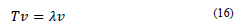
Because T is not necessarily symmetric, it does not have orthonormal eigenvectors. The following transformation is performed:
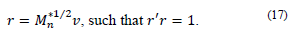
Then:
It is important to mention that matrix T*n.n is constructed considering the available data principle and that from this matrix, the eigenvalues λ and eigenvectors 𝑟 are found.
A more important situation in this procedure is that the eigenvalues λ in spaces Rp are Rn are equivalent, which makes the transition relations valid and provides coordinates Ψ and φ.
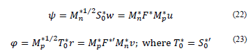
3.5. Transition relations
As mentioned above, the MCAadp method guarantees that the eigenvalues in spaces Rn and Rp are equivalent; in this way, we can relate the coordinates of one space with the coordinates of another, considering the following expressions:
3.6. Components in Rn and Rp
To perform the calculations of components Ψn,p in Rp, the point product of matrix S0* with the eigenvector associated with the space of variables
 is performed. To calculate components φp,p in Rn, the point product of matrix T0* with the eigenvector associated with the space of individuals
  is performed. Based on these calculations, the following expressions are obtained:
3.7. Inertia expressions for available data
Presented in this section are the expressions of Total Inertia, Inertia by category, and Inertia by question, such that these expressions consider that the available data principle 𝑠 ∗ is used; it is the marginal estimated by row and is replaced in each Inertia expression. The new expressions are presented as follows:
Total Inertia: This inertia depends on the existing number of data with NA. If there are more, then s* is smaller and thus the Total Inertia increases.
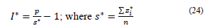


where p q is the number of categories per question q.
4. Equivalence between the results of the MCAadp and the MCA of incomplete tables
In the MCAadp proposal, the sums of the rows of the disjunctive table with missing data are replaced by the constant
 to calculate the inertias. In addition, the sums and point products of the disjunctive table with missing data are equivalent to the same operations with the incomplete disjunctive table (i.e., with 0 instead of NA). Thus, the MCAadp coincides with the MCA method for an incomplete disjunctive table [7].
In these methods, the MCA properties are retained. The advantage of the MCAadp is derived from the NIPALS algorithm, which sequentially obtains the factors, leading to shorter calculation times if only the axes that will be analyzed are obtained.
5. Application
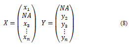
The DogBreeds database contains 27 breeds and six qualitative variables: Size (SIZ), Weight (WEI), Speed (SPE), Intelligence (INT), Affection (AFF), and Aggressiveness (AGR). Each variable has two or three categories, as illustrated in the FactoClass package [17]. SIZ has three categories: big, medium (med), and small. WEI has three categories: heavy, medium (med), and light. VEL has three categories: fast, medium (med), and slow. Variable INT has three categories: high, medium (med), and low. AFF and AGR each have two categories: high and low. It is important to mention that these qualitative variables are used as indicator variables. In this manner, the study is performed in a data matrix Z ij , which contains one, zero, or NA, depending on if the category is present or absent or if there are missing data. It is important to mention that matrix Z ij is of dimension n*p where n represents individuals and p represents categories.
5.1. Missing data simulation in the study case
The work is performed with the first six variables and missing data will be randomly assigned to the matrix. In the following structure of the R software, m corresponds to the position where the missing data is located and a corresponds to the percentg of missing data values of the total
fmd <- function(Xo,a)
{
X. <- as.matrix(Xo)
n <- nrow(X.); p <- ncol(X.); N <- n*p
m <- sample(N, round(a*N,0)) ; d <- length(m)
for(j in 1:d){
X.[m[j]] <- NA
}
return(X.)
}
5.2. Simulation study
Table 3 shows the proposed simulation scenarios, which have a missing completely at random (MCAR) mechanism. At the same time, the scenarios when the entire data matrix has 1, 2, or 3 NA per row are considered. In the first three scenarios, the marginal per row Z i is constant for every i. However, when there are from 0 to 1, 0 to 2, and 0 to 3 NA per row, the marginal per Zi is not constant for every i. It is important to mention that the marginal per column is not constant for the j categories.
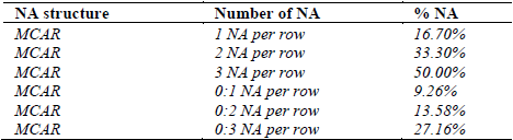
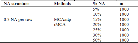
It is also important to mention that the NA percentage is calculated based on the total number of records (27 ∗ 6). In this article, the work is performed with a maximum of 50% of missing data; the NA percentage in the last three scenarios is randomly generated. To study the presence of NA in a more general and random manner, different simulations were performed, as shown in Table 4, where the records per individual will have a maximum of three NA per row (not exceeding 50%). One thousand matrices are generated for each NA percentage: 5%, 10%... 50%, i.e., there will be 7000 simulated matrices and they are compared with the complete data case.
5.3. Statistical analysis of the simulation scenarios
First, the matrix with complete data must be analyzed to see how each of the following indicators behave:
Eigenvalues λ and eigenvectors u
Components Ψ and φ in Rn and Rp
Total Inertia, Inertia by category, and Inertia by question
Descriptive power (λ1 + λ2) / Σ λ
Factorial planes
Orthogonality in the components and orthonormality in the eigenvectors
With this starting point, the same indicators are analyzed for each of the scenarios proposed in Table 3. In each of these analyses, it is identified if the inertia expressions agree with the theory with complete data. Then, in section 6, a comparison is performed between the MCAadp and the imputation method, where the scheme of Table 4 is used and where 𝑚 is equal to the number of matrices to simulate the structure.
The code developed in the R software using the MCAadp method can be viewed at the following website: https://github.com/AndresOchoaRSA/MCAapd
To perform the factorial planes, the s.label() function of the ade4 library was used [6]. For the analysis with the imputation method, the missMDA library was used [10]. The R software version used is 3.6.1.
6. Results
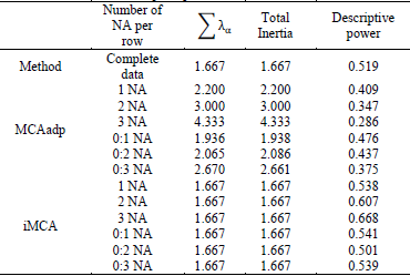
Presented in Table 5 is a comparison of the previous scenarios with the imputation method proposed by Josse, J. et al. [12]. It is observed that the Total Inertia with the MCAadp is higher compared to the complete data. With the imputation method (iMCA), the Total Inertia is the same as in the complete data. This occurs because the imputation delivers an imputed complete matrix, where the inertia expressions are the same. However, it is observed that the descriptive power in the MCAadp method decreases, whereas with the imputation method it increases as a function of the number of NA. This may be considered a drawback of the imputation method, since an increase in descriptive power implies that having more NA records would be a favorable situation; however, it is expected that by having more NA in a data matrix, the representation performed will lose its descriptive power.
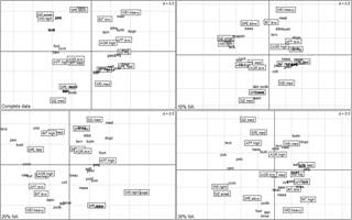
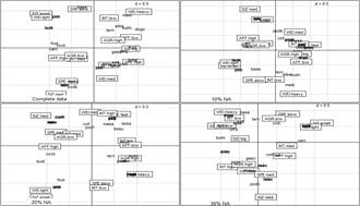
Figure 1 illustrates four first factorial planes of these analyses: MCA with complete data and MCAadp with 10%, 20% and 30% of NA. It is observed how as the missing data increase, some typologies and features that were found in the complete data are lost. However, Figure 2 shows the comparison between the complete data and matrices with missing data where the iMCA was used. It is observed that some typologies are also lost when the number of missing data points increases. This type of analysis with the factorial planes becomes more difficult because it is a visual analysis and there should be an indicator describing the characteristics of the variables and individuals in these two axes. The proposed indicator is the descriptive power (λ1 + λ2) / Σ; with such an indicator, the percentage of variance explained in those two axes is found.
Source: The Authors
Figure 1 Factorial plane comparison: complete data, MCAadp with 10%, 20%, and 30% of NA.
Source: The Authors
Figure 2 Factorial planes comparison: complete data, iMCA with 10%, 20%, and 30% of NA.
For this simulation case, Figure 3 shows that as the amount of missing data increases, the descriptive power decreases with the MCAadp method. Conversely, with the iterative MCA, as the missing data percentage increases, the descriptive power decreases. The previous situation is considered to be inconsistent because when there is a larger amount of missing data, the inertia relationships present in the data set should be more difficult to explain. It is important to mention that the line of reference corresponds to the descriptive power with complete data, which is 0.5198.
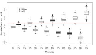
Source: The Authors
Figure 3 Behavior of the descriptive power as a function of the NA percentage with MCAadp and iterative MCA (iMCA)
Note that for the case of MCA with complete data, the marginal per row is equal to 𝑠 and in the case of MCAadp it is s*, where s > s* → I < I * , i.e., the inertia I* in the MCAadp is higher than in MCA; however, as observed in Figure 3, the inertia in the first factorial plane decreases as a function of the NA percentage.
7. Conclusions
Based on the results, the MCAadp presents a practical and efficient solution because its programming is simple and it has the interesting properties of orthogonality in the components, orthonormality in the eigenvectors, and equivalence in the eigenvalues in Rp and Rn, among others [15].
The MCAadp is an alternative solution to the missing data problem. It resorts to imputation techniques, but the user can use the method to perform imputation via the reconstitution of the matrix. In comparison with the iterative MCA method, the MCAadp presents higher consistency in terms of descriptive power, because at a higher number of NA, the descriptive power is expected to decrease. However, it is important to consider comparisons with other methods such as the regularized iterative MCA method [11] or the MCA with multiple imputations [3].
In a Masters thesis [15], work was also done with a higher-dimension data set (tea consumption data), and the same results were found regarding the simulation process, i.e., the descriptive power decreases as the missing data percentage increases when using MCAadp. For future works, it would be interesting to perform a cluster analysis and a multiple factorial analysis for qualitative variables, both with missing data via PLS, and adapt them to current libraries of the R software.

