


 English (pdf)
 Article in xml format
 Article references
 Send this article by e-mail
 Cited by SciELO
  Cited by Google
  Similars in
SciELO
Similars in
SciELO  Similars in Google
 Permalink
1. INTRODUCCIÓN
We know since the early works of Albert Atterberg (1846-1916) and Arthur Casagrande (1902-1981) that the plasticity of fine-grained soils resembles a fundamental characteristic of them [1,2]. In this sense, the consistency of such soils varies with increasing moisture content from solid, semi-solid, plastic, and liquid states, coined the arbitrary borders between them as the shrinkage limit, the plastic limit (𝑊𝑝), and the liquid limit (𝑊𝑙), respectively [3]. Moreover, the difference between 𝑊𝑙 and 𝑊𝑝 is named Plasticity Index (𝑃𝐼). Together with its granulometric analysis, the determination of the plasticity of the soil allows it to be classified according to international systems, such as the USCS [4] and the AASHTO [5,6], among other technical applications in soil science. There are various laboratory methods for determining 𝑊𝑙, such as that of the Casagrande device [7] or through penetrometer tests [8], as well as a method for the determination of 𝑊𝑝 [7]. Nevertheless, it is unknown until date, a static, multisampling, and automatic test able to determine directly 𝑊𝑙, 𝑊𝑝, and 𝑃𝐼, with a single measure. In this sense, the method developed by [9] needs two measures, subjecting sieved samples to different suction pressures of −1,500 KPa (𝑝𝐹4.2) and −33 KPa (𝑝𝐹2.5) inside pressure-membrane extractors [10].
Regarding Wl measurements, made with the percussion-cup test method, [11] showed that they can vary depending on the technician using them, whether they are performed in different laboratories as well as the device used, or the material in which the cup hits. The correct calibration of the device, the cadence of hitting, and the used grooving tool also have an impact on this reproducibility [12]. Besides, greater reproducibility of the results was found in tests carried out with penetrometers [8]. Regarding the determination of Wp using the rolling test, [11] showed that its reproducibility is even lower than that obtained for Wl, which shows a subjective component in the measurements. Moreover, [13] stated that Wp is a measure of soil brittleness. These authors also revealed that this behaviour depends on the continuity of water circulation into the soil rods, and therefore, cavitation occurs. To follow up, PI is related to friction and permeability in fine-grained soils. In this regard, friction in soils decreases when PI increases whereas permeability exhibits contrary behaviour [14]. Next, based on the instructions of [15,16] to classify soils, become tacitly and qualitatively deduced that the ability of a soil to retain water increases with its plasticity through a characteristic called dilatency, performed by means of simple and well-known procedure. Besides, [17] established that
2. Materials and methods
The laboratory and data analysis techniques used as well as the geological locations of the soil samples analysed are described below.
2.1. Geological and geographical locations of the samples
The samples were obtained from the towns of Vélez-Málaga, Granada, Jaén, Linares, Baza, and Caravaca de la Cruz, belonging to the Betic Cordillera (Spain). The geotechnical classifications along with other characteristics are collected in the Table 1; each location is signified by the first letter of its initials, as shown in Fig. 1.
Table 1 Experimental results for the samples analysed.
| Soil | Wl (%) | Wp (%) | pF25 (%) | pF42 (%) | PI (%) | F (%) | USCS | AASHTO | GI |
|---|---|---|---|---|---|---|---|---|---|
| J1 | 44.0 | 20.4 | 27.6 | 18.3 | 23.8 | 92.1 | CL | A-7-A-7-A | 20 |
| J2 | 34.8 | 18.8 | 23.3 | 10.3 | 15.9 | 91.0 | CL | A-6 | 9 |
| G1 | 41.1 | 25.7 | 26.4 | 16.5 | 15.4 | 96.3 | ML | A-7-A-7 | 1 |
| G2 | 36.8 | 18.4 | 23.7 | 12.4 | 18.3 | 89.4 | CL | A-6 | 15 |
| G3 | 36.6 | 18.6 | 26.4 | 12.7 | 17.9 | 91.1 | CL | A-6 | 13 |
| G4 | 42.8 | 20.9 | 26.1 | 15.1 | 21.9 | 93.7 | CL | A-7-A-7 | 21 |
| VM | 28.4 | 27.0 | 23.5 | 10.9 | 1.43 | 41.9 | SM | A-2-4 | 0 |
| L1 | 30.1 | 23.9 | 17.9 | 7.5 | 6.20 | 84.2 | ML | A-4 | 4 |
| C1 | 52.4 | 26.1 | 25.6 | 15.1 | 26.2 | 88.1 | CH | A-7-A-7-A | 20 |
| C2 | 37.8 | 23.2 | 23.7 | 12.0 | 14.6 | 63.1 | SC | A-2-6 | 0 |
| C3 | 38.7 | 25.0 | 25.7 | 15.5 | 13.7 | 82.6 | SM | A-6 | 3 |
| C4 | 41.5 | 17.3 | 24.1 | 14.3 | 24.2 | 98.0 | CL | A-7-A-7-A | 11 |
| C5 | 40.3 | 24.5 | 23.9 | 14.3 | 15.7 | 95.5 | CL | A-7-A-7-A | 8 |
| C6 | 43.5 | 22.8 | 23.5 | 15.3 | 20.7 | 89.5 | CL | A-7-A-7-A | 15 |
| C7 | 50.5 | 25.8 | 25.9 | 16.3 | 24.7 | 87.5 | CH | A-7-A-7-A | 14 |
| J3 | 47.3 | 24.4 | 24.7 | 14.3 | 22.9 | 96.2 | CL | A-7-A-7-A | 20 |
| J4 | 46.6 | 23.7 | 27.0 | 15.4 | 22.8 | 96.9 | CL | A-7-A-7-A | 26 |
| J5 | 61.8 | 25.7 | 28.9 | 18.0 | 36.1 | 99.3 | CH | A-7-A-7-A | 42 |
| B1 | 29.1 | 19.1 | 22.4 | 10.2 | 10.0 | 85.5 | SC | A-6 | 2 |
| B2 | 32.6 | 18.2 | 23.3 | 10.3 | 14.4 | 97.4 | CL | A-6 | 14 |
| B3 | 26.0 | 20.6 | 22.7 | 6.4 | 5.4 | 58.7 | CL-ML | A-4 | 0 |
| B4 | 32.2 | 18.1 | 24.2 | 9.6 | 14.1 | 97.6 | CL | A-6 | 14 |
| B5 | 45.7 | 19.7 | 28.7 | 16.7 | 25.9 | 97.6 | CL | A-7-A-7-A | 27 |
Source: self-made.
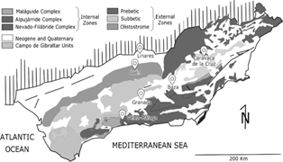
Source: simplified scheme of Sanz de Galdeano et al., 2007.
Figure 1 Geological locations of the samples in the Betic Cordillera.
The Betic Cordillera is located in the south-east of Spain, in a sloping strip that extends from Cádiz to the Balearic Islands, and they constitute the westernmost Alpine Mountain chain in the Mediterranean, beside the Rif [20].
2.2. Laboratory techniques
In the next sections, we describe W1, Wp, and
2.2.1. Atterberg limits measurement
All the soils analysed were extracted via undisturbed sampling using a push-in Shelby tube sampler with a 101.6 mm inner diameter and a 1.63 mm wall thickness. They were delivered undisturbed to a testing laboratory into PVC pipes, in which we classified the soils, performed granulometry, and determined the liquid limit and plastic limit of the samples.
With a part of the sample, granulometry was performed through sieving following the NLT 104/91 standard [4].
The second part of the sample was sieved with an N40 ASTM sieve to determine the Atterberg limits, and the sieved fraction was separated into two portions by quartering. With the first half, we applied the Casagrande device method, which allowed us to determine W1 following the ASTM D 4318-84 standard [19].
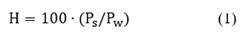
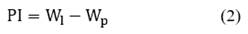
Next, the moisture of the precise part of the sample that slid into the groove was measured by oven-drying at 105°C, expressed as weight percentage (H), by weight difference before (Pw) and after drying (Ps), following eq. (1).
On the other hand, the plastic limit (Wp) is determined by ASTM D 4318-84 standard [19].
In addition, PI is defined by [19] as the difference between W1 and Wp (eq. 2).
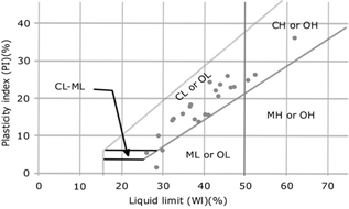
Once determined W1 and PI of each sample, the Casagrande plasticity chart allows to classify the soils according to its plasticity (see Fig. 2). Consequently, with granulometry, W1 and PI, the soils were classified using the USCS [5] and AASHTO [6] systems.
2.2.2. Soil water holding capacity
To clarify some aspects about the pressure-membrane extractors used in this study, the matric potential (F) represents the tension that soils exert in sorption phenomena. In this regard, [21] defined
In this paper, we assume the generalized Soil Water Retention Curve (SWRC) equation described by [21]. In this model, water is covering the mineral surfaces because of water adsorption phenomena and capillary effects in pores with different diameters. This is represented in eq. (4):

where total water retained (θ) equals adsorbed water (θ a ) plus capillary water (θ c ) under ψ prevailing suction.
The adsorbed water mainly depends on the specific surface area of the minerals of the soil as well as the cation exchange capacity (CEC) of its clays, colloids, and organic matter [23,24]. This moisture, according to the BET theory [25] could be represented as a multilayer of sorbito, covering the solid phase of a soil, where Van der Waals forces, electrically charged particles, osmotic and hydration components are involved [26].
Furthermore, [27] computed for adsorbed water θa (ψ) with eq. (5):
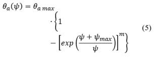
where ψ is the suction pressure, θa max is the adsorption capacity, ψmax is the higher matrix suction, and
Moreover, [27] also determined in eq. (6) the capillary water retention θc (ψ), given by the following equation:
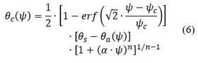
It depends on porosity or saturated water content (θs), air entry suction (α -1), pore size distribution (n), and mean cavitation suction (ψc).
Moreover, water sorption-desorption curves are affected by hysteresis, yielding that θ(ψ) is greater when the soils absorb moisture than when drying [28]. Thus, the samples were tested before saturation.
To sum up, when we subject a saturated sample to suction pressures of −1,500 KPa, a fraction of water is absorbed through the porous disk of the Richards apparatus used. So that it will contain adsorption moisture and water in pores up to 0.2 μm in diameter [29]. On the other hand, saturated samples subjected to −33 KPa, contain the moisture retained at −1,500 KPa plus the slow-flow gravitational water, which remains in pores between 0.2 and 8 μm in diameter [29]. Likewise, [30] relate shear strength with SWRC for unsaturated soils. Moreover, as W i is determined with shear strength-based tests and W p is related to cavitation [13], we measure soil water holding capacity next.
2.2.3. Soil water holding capacity measurement
Soil water holding capacity is measured with a Richards extractor. This is a device made up of hermetic circular chambers containing 300 mm porous porcelain plates with membranes. It could probe the samples by applying different suction pressures using a compressor, pipes, and gauges [10].
With more detail, the porcelain disks were saturated in deionized water for 24 hours. Then two quartered batches were taken from the dry soil samples, previously sieved with an ASTM N40 sieve. Later, those samples were placed carefully in rubber rings on the porcelain disks. Next, deionized water was poured onto the porcelain disks and they were left to rest in expanded polystyrene chambers for 2 days so that they could absorb the moisture. Subsequently, both batches of soil samples were subjected to the required suction pressure for 2 days into independent chambers of the Richards extractor. The water that the samples did not retain was evacuated through these porous disks and membranes. Finally, the moisture retained by the samples after the process was determined by weight difference by drying in an oven at 105°C, according to eq. (1). For this, weights substances with a lid, spatulas, and washing bottles were used.
In this work, the prevailing suctions used (ψ) were −1,500 kPa (pF = 4.2) and −33 kPa (pF = 2.5), respectively. As a consequence, the moisture content of a soil expressed as a percentage by weight at probed pressure will be denoted as pF 4.2 and pF 2.5 in tables and machine-learning model equations.
3. Calculation
For data analysis, SPSS 25 [31] and a Multiple Classifier System (MCS) are used together [32, 33]. MCSs combines regression algorithms from heterogenous theoretical backgrounds programmed with Python 3.0 [34]. So that we used the Pandas [35], Seaborn [36], Matplotlib [37], Scikit-learn [38], and Statsmodels [39] libraries. The commented source code is suitable for the Jupyter Notebook environment [40]. The starting data in CSV format and a code example can be consulted in the GitHub repository that is cited in the appendix A. Those techniques were Multiple Linear Regression (MLR), Decision Tree Regression (DTR), Random Forest Regression (RFR), and Support Vector Machines Regression (SVMR).
First, MLR is coded since it provides intelligible models. In this regard, [41] implemented MLR models according to eq. (7):

which represents a linear model of coefficients w = (w0, w1, … wn) and characteristics X = (x1, x2, … xn), where  is the variable predicted by the model.
To do this, scikit-learn [41] minimises the residual of the sum of squares between the observed objective characteristics and those predicted by the linear model, solving the following minimizing function (8):
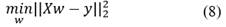
On the other hand, the Statsmodels library [39] implements the ordinary least squares technique capable to fit the data model, providing additional statistical parameters used in our MCS. Furthermore, the parameters of the models and their statistical adjustments were evaluated, bearing in mind a level of statistical significance α = 0.05.
Besides, DTR was implemented with scikitlearn. Briefly, DTR algorithms generate recursive partitions of the feature space, following rules that maximize the differentiation of the splits. Such splits set the nodes of a tree structure. So that, a DTR model learns local linear regressions on the basis of such nodes [41]. The depth of the tree was set by default in the code.
Moreover, using scikit-learn, the RFR technique was implemented. So, 100 of the previously said decision trees were selected, taking different subsets of the whole original dataset, and then, two estimators of the predictive accuracy were obtained by averaging. This time, Root Mean Square Error (RMSE) and Mean Absolute Error (MAE) were computed to control over-adjustment, yielding better predictive capability than a DTR [42]. On the contrary, DTRs may provide intelligible models [41].
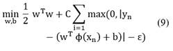
Next, SVMR capabilities were provided to the code using scikit-learn. So that, bearing in mind eq. (7), where w0 = b, the aim is to find a function as flat as possible with the most ε deviation from the training data [43], computed as in eq. (9). In this sense, C is a regularization parameter and ϕ is a linear kernel function.
To sum up, following [44] we perform MLR with the whole dataset to establish explainable empirical relationships for W
l
, W
p
, and PI to choose the characteristics of the models. Once selected the characteristics of each model, the beforementioned four regression techniques are used to predict W
l
, W
p
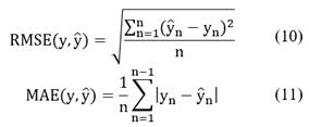
, and PI. Then, using scikit-learn and following [45, 46], a K-folded double cross-validation score with K = 10 is computed in terms of RMSE (eq. 10) and MAE (eq. 11), to estimate the accuracy of the candidate models. In this sense, K-folded cross-validation is implied to split n observations into K equal subsets so that the (k - 1)/k fraction of the observations is used for model construction, while the 1/k portion of the data is used for validation. In eq. (10, 11), n is the number of observations,  the predicted values of the model, and y
n
the observed values.
the predicted values of the model, and y
n
the observed values.
4. Results
Before continuing, we must show that the analyzed samples had a higher concentration of materials that passed through an N200 ASTM sieve than the starting soils because to determine the Atterberg limits, the samples were sieved with an N40 ASTM sieve. That is why we must define the
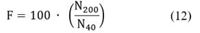
Later, Table 1 summarises the experimental results obtained. The quantities are expressed as percentages by weight. W1 is the liquid limit. Wp is the plastic limit. The water retained at −33 KPa is pF25. The water retained at −1,500 KPa is pF42. PI is the plasticity index. F is the calculated portion of soil particles in a sample sieved with an N40 ASTM sieve that passes through an N200 ASTM sieve. USCS is the classification of the soil samples in the USCS system. AASHTO is the classification of the soil samples in the AASHTO system with the group index (GI).
Next, in Fig. 2, the analysed samples are presented, following the USCS system. Of the 23 soils, three are high-plasticity clays (CH), two are low-plasticity silts (ML), one is a low-plasticity clayey silt (CL-ML), and the remaining 17 are low-plasticity clays (CL).
After, non-parametric linear correlation tests were performed among the study variables (model characteristics) with SPSS 25. Said correlation coefficients were taken into account to preselect the characteristics to be used in the construction of the models, with certain precautions. Table 2 summarises the results obtained after applying Spearman’s ρ test.
Table 2. Spearman’s ρ correlation coefficients and level of bilateral significance.
| N = 23 in All Cases | Wl | Wp | PI | pF2.5 | pF4.2 | F | |
|---|---|---|---|---|---|---|---|
| Wl | Correl. | 1.000 | 0.375 | 0.915** | 0.732** | 0.838** | 0.439* |
| Next (bilat.) | . | 0.078 | <0.001 | <0.001 | <0.001 | 0.036 | |
| Wp | Correl. | 0.375 | 1.000 | 0.077 | 0.222 | 0.399 | −0.348 |
| Next (bilat.) | 0.078 | . | 0.727 | 0.308 | 0.059 | 0.104 | |
| PI | Correl. | 0.915** | 0.077 | 1.000 | 0.684** | 0.713** | 0.540** |
| Next (bilat.) | <0.001 | 0.727 | . | <0.001 | <0.001 | 0.008 | |
| pF2.5 | Correl. | 0.732** | 0.222 | 0.684** | 1.000 | 0.851** | 0.534** |
| Next (bilat.) | <0.001 | 0.308 | <0.001 | . | <0.001 | 0.009 | |
| pF4.2 | Correl. | 0.838** | 0.399 | 0.713** | 0.851** | 1.000 | 0.364 |
| Next (bilat.) | <0.001 | 0.059 | <0.001 | <0.001 | . | 0.088 | |
| F | Correl. | 0.439* | −0.348 | 0.540** | 0.534** | 0.364 | 1.000 |
| Next (bilat.) | 0.036 | 0.104 | 0.008 | 0.009 | 0.088 | . | |
Source: self-made.
5. Discussion
First, we will use the information in Table 2 to select the appropriate characteristics to build the models, avoiding collinearities between them. Such is the case between pF2.5 and pF4.2, (ρ = 0.851; p. < 0.001), so they will not be included in the same model. However,
Consequently, pF2.5 and pF4.2 can be selected to build single-feature models, and F and pF4.2 can be selected for two-feature models. To avoid over-adjustments, models that do not use powers of any of their characteristics have been chosen, especially when the range of values of the liquid limit of the samples is limited (from 26 to 62). Further, the adjustments to a linear model seem adequate.
5.1. Determination of the liquid limit
Table 2 shows that the linear correlations between the liquid limit (W1) and the variables pF2.5 (ρ = 0.732; p. < 0.001), pF4.2 (ρ = 0.838; p. < 0.001) and F (ρ = 0.439; p. = 0.036) are significant, with a confidence level greater than 95% in all cases. Consequently, characteristics F, pF2.5, and pF4.2 were selected to build linear models with a single characteristic, whereas
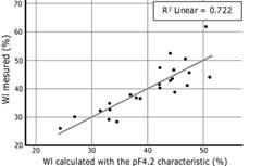
Considering the data collected in Table 5, the model with a unique characteristic pF4.2 has been selected since it is the only one in which all of its coefficients are statistically significant, with a confidence level of at least 95%. It also presents a considerable adjustment expressed as R2 (0.722) and is statistically significant, with a confidence level greater than 99%. The fit between the measured
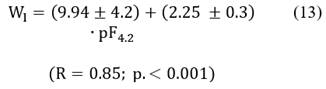
Table 3 Linear models studied to determine Wl.
| Characteristics of the Model | Coefficients | Std. Err. | P > |t| | R2 and Next Change in F |
| F | W0 = 13.31 W1 = 0.31 |
10.0 0.1 |
0.199 <0.013 |
0.258 (p. = 0.013) |
| pF4.2 | W0 = 9.94 W1 = 2.25 |
4.2 0.3 |
0.028 0.001 |
0.722 (p. < 0.001) |
| pF2.5 | W0 = −23.9 W1 = 2.58 |
13.8 0.6 |
0.099 <0.001 |
0.505 (p. < 0.001) |
| pF4.2 F | W0 = 4.85 W1 = 2.07 W2 = 0.08 |
6.3 0.3 0.1 |
0.448 <0.001 0.290 |
0.737 (p. < 0.001) |
Source: self-made.
Source: self-made.
Figure 3 Fit of the selected model to determine the liquid limit (Wl). Measures expressed as percentages by weight.
Table 4 Different liquid limit models scores with the
| Regression model | Mean RMSE | Mean RMSE Standard deviation |
|---|---|---|
| MLR | 4.15 | 2.73 |
| DTR | 7.06 | 2.98 |
| RFR | 6.03 | 2.88 |
| SVMR | 3.65 | 2.92 |
Source: self-made.
Table 5 Proposed model to determine PI.
| Characteristics of the Model | Coefficients | Std. Err. | P > |t| | R2 and Next Change in F |
| F | W0 = −14.45 W1 = 0.37 |
7.9 0.1 |
0.080 <0.001 |
0.451 (p. < 0.001) |
| pF4.2 | W0 = −7.72 W1 = 1.92 |
4.4 0.3 |
0.096 <0.001 |
0.628 (p. < 0.001) |
| pF2.5 | W0 = −41.99 W1 = 2.42 |
12.3 0.5 |
0.003 <0.001 |
0.531 (p. < 0.001) |
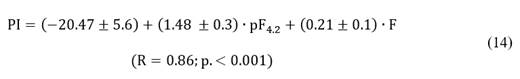
| pF4.2 F | W0 = −20.47 W1 = 1.48 W2 = 0.21 |
5.6 0.3 0.1 |
0.002 <0.001 0.007 |
0.745 (p. < 0.001) |
Source: self-made.
In Table 4, we can see the scores of MLR, DTR, RFR and SVMR models calculated as the mean RMSE of a cross-validation procedure with 10 K-folds.
The SVMR model exhibits the lower mean RMSE (4.15) followed by MLR model (4.15), but the MLR model has an inferior standard deviation (2.73) vs (2.92). DRT and RFR demonstrate the worst scores. On the other hand, [11] established the tolerance limits in the reproducibility required for the determination of the liquid limit in ±5% for control processes and in ±10% for design work. Accordingly, MLR and SVMR models would be acceptable for design purposes.
5.2. Determination of the plasticity index
Table 2 shows that the linear correlations between the PI and the variables pF2.5 (ρ = 0.684; p. < 0.001), pF4.2 (ρ = 0.713; p. < 0.001), and F (ρ = 0.540; p. = 0.008) are significant, with a confidence level greater than 99% in all cases. Consequently, the characteristics F, pF2.5, and pF4.2 were selected to build linear models of a single characteristic, and F and pF4.2 were selected for a model of two characteristics, which are reflected in Table 5.
In view of the data collected in Table 5, the model with the characteristics pF4.2 and
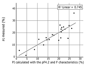
Next, in Table 6, we show the scores of MLR, DTR, RFR and SVMR models calculated as the mean RMSE of a cross-validation procedure with 10 K-folds.
Table 6 Different plasticity index models scores with pF4.2 and F characteristics and double Cross-validation (K=10) in terms of mean RMSE with mean standard deviation.
| Regression model | Mean RMSE | Mean RMSE Standard deviation |
|---|---|---|
| MLR | 3.81 | 2.36 |
| DTR | 5.93 | 3.41 |
| RFR | 4.41 | 2.26 |
| SVMR | 4.04 | 2.31 |
Source: self-made.
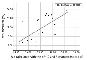
Table 7 Proposed model to determine
| Characteristics of the Model | Coefficients | Std. Err. | P > |t| | R2 and Next Change in F |
|---|---|---|---|---|
| pF4.2 F |
W0 = 25.32 W1 = 0.60 W2 = −0.13 |
3.5 0.2 0.04 |
<0.001 0.006 0.009 |
0.380 (p. = 0.008) |
Source: self-made.
This time, the MLR model exhibits the lower mean RMSE (3.81) followed by SVMR model (4.04), but the SVMR model has an inferior standard deviation (2.31) vs (2.36). DTR and RFR have the worst scores and they are not considered, because DTR models showed over-adjustment without cross-validation (RMSE = 0). Although [11] did not establish an acceptable tolerance margin for the determination of PI, and this measure carries, by definition, the errors in the determination of W1 and Wp, the tolerance margins that this researcher considered acceptable for the measurement of W1 will be selected as reference, as the most restrictive. Accordingly, MLR and SVMR models would be acceptable for design purposes (±10%).
5.3. Determination of the plastic limit
In order to determine Wp we have selected pF4.2 and
In this regard, the model is defined by eq. (15), to the detriment of indirect measurement, since it carries the errors of the determinations of W1 and PI. Further, W1 and Wp are determined with very different standards and methods. In this way, using the whole dataset, the following experimental relation is achieved (eq. 15):
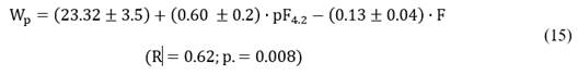
Next, the fit between the measured Wp values and those calculated by means of eq. (15) are presented in Fig. 5.
Subsequently, in Table 8, we collect the scores of MLR, DTR, RFR and SVMR models with pF4.2 and F characteristics, calculated as the mean RMSE of a cross-validation procedure with 10 K-folds.
Table 8 Different plasticity index models scores with pF4.2 and F characteristics and double cross-validation (K=10) in terms of mean RMSE with mean standard deviation.
| Regression model | Mean RMSE | Mean RMSE Standard deviation |
|---|---|---|
| MLR | 2.47 | 0.91 |
| DTR | 3.57 | 1.34 |
| RFR | 2.64 | 1.46 |
| SVMR | 2.32 | 1.30 |
Source: self-made.
Now, the SVMR model exhibits the lower mean RMSE (2.32) followed by MLR model (2.47), but the MLR technique yields an inferior standard deviation (2.31) vs (2.36). DRT and RFR show higher scores and exhibit over-adjustments without cross-validation (RMSE = 0), so they are rejected. Moreover [11] found a tolerance margin of reproducibility for the rolling test method of ±10% for control purposes. Therefore, using pressure-membrane extractors offers an acceptable uncertainty, especially when all of them are below a tolerance margin of ±5, so MLR and SVMR models appear very precise. Furthermore, [47] found an uncertainty of ±20% in the determination of
6. Conclusions
The aim of this study was to develop an alternative method suitable for the determination of Atterberg limits using a pressure-membrane apparatus and MCSs.
In addition, tree models have been described using MLR and SVMR techniques that would allow the determination of W1, Wp, and PI in the analysed soils. In this regard, the selected characteristics were pF4.2 and F. The tolerance margins shown for W1 and PI seem appropriate for design purposes. On the other hand, in the determination of Wp, we have found appropriate tolerance margins for control work.
Likewise, in view of the experimental results, machine-learning techniques simplify the method proposed by [9], offering models that conceptually make sense with respect to the Atterberg limits. Thus, Wp, and PI increase proportionally as the capacity to retain water strongly bound to the soil particles and in pores with a diameter less than 0.2 μm increases. In contrast, the amount of fine material with a maximum diameter of less than 0.074 mm also affects these plasticity indices but to a lesser extent. However, estimating the liquid limit only requires measuring the capacity of the samples to retain water in fine pores smaller than 0.2 μm and form films around their mineral grains (pF4.2), and we have found that the first increases with the second.
Furthermore, while the precision of the method could be improved in later studies, using it could entail certain advantages. For instance, it allows several static tests of different samples to be carried out at the same time, eliminating subjectivity in the determinations and increasing the productivity of the laboratories. Likewise, it could prevent the need to carry out such frequent trial-error tests in standardized methods if it is used as an indicative test of the moisture required for the determination of W1, Wp, and PI. Besides, cheaper methods may be developed.

