


 English (pdf)
 Article in xml format
 Article references
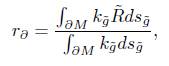
 Send this article by e-mail
 Cited by SciELO
  Cited by Google
  Similars in
SciELO
Similars in
SciELO  Similars in Google
 Permalink
1. Introduction
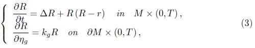
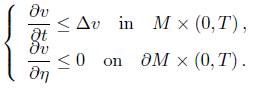
There is no need to talk about the importance of the Ricci flow (on closed and noncompact manifolds without boundary) in geometric analysis and low dimensional topology. Moreover, besides its numerous applications in geometric analysis, another of the great merits of studying the Ricci flow is that it gives a way of understanding the behavior of certain nonlinear parabolic equations using geometric insights. The subject of this paper is the study of the following boundary value problem for the Ricci flow on a surface with boundary:
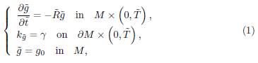
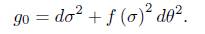
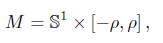
where  is the geodesic curvature of the initial metric and M is a surface homeomorphic to a cylinder
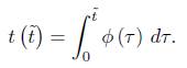
  . We shall also consider the corresponding boundary value problem for the normalised version of (1). Recall that the normalised flow is obtained from (1) by the following procedure. Let
  be a function such that
  so that the area A
g
(M) of the surface M with respect to the rescaled metric g is kept equal to 1 at all times. Then the time parameter is rescaled by setting
so that the area A
g
(M) of the surface M with respect to the rescaled metric g is kept equal to 1 at all times. Then the time parameter is rescaled by setting
By this procedure we obtain the following boundary value problem:
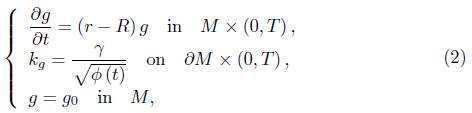
Where
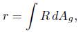
is the average scalar curvature. From now on, all quantities referring to the un-normalised flow (1) will have a tilde, whereas those referring to the normalised flow (2) will not.
The existence theory for the unnormalised flow, and hence that of the normalised flow, is well known and we refer to the introduction of [3] for a short discussion on the matter. Hence, in this work, we shall be concerned with the asymptotic behavior of both versions of the flow under certain geometrical assumptions, and, to give the reader a certain feeling of anticipation, we must say that what actually prompted us to write this note is how curious this asymptotic behavior appears to be; we can even say that we have been rewarded by finding out some unexpected (at least to us) results. We refer to some of our results as unexpected, because we were guided by the following principle: the behavior of the flow in surfaces with boundary must parallel that of the flow in closed surfaces (and the results of Brendle in [1] seems to give some support to it). This principle turned out to be wrong.
Indeed, under the assumption that  , we shall prove long time existence results for both the normalised and unnormalised flow, but we will show that whereas in the normalised flow the curvature remains uniformly bounded (at least in a set of examples we consider, see Section 4.1), in the unnormalised flow it blows up in infinite time; this already marks a difference between the case of a cylinder and the corresponding case of closed surface of zero Euler characteristic, where both the normalised and unnormalised flow are the same. This, of course, has to do with the fact that Rg0 > 0 is not a possibility in the case of closed surfaces of Euler characteristic zero.
To continue with the surprising behavior we encountered, we show that even though we expect the curvature to converge towards zero, it does not do it exponentially, contrary to what does happen in the case of closed surfaces. The authors think both result are interesting enough to merit reporting them; besides the proofs are elementary, and this may be of interest to the non specialist, and to those also interested on the behavior of nonlinear parabolic equations.
Let us now be more precise regarding the results we shall prove in this paper. We begin with our longtime existence result.
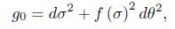
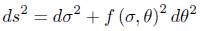
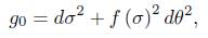
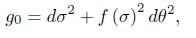
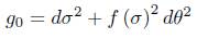
Theorem 1.1. Assume that the initial metric has the form
and that Rg0 ≥ 0 and kg0 ≤ 0. Then the normalised and the unnormalised flow exist for all time.
We show the previous result for the normalised flow for initial data of the form  in Section 3, and in Section 4 we show that whenever the normalised flow exists for all time so does the unnormalised flow (no symmetry assumptions are required to prove this claim). This result should be compared with Proposition 2.3 in [3], where it is shown, in the case of a disk, that under the conditions R
g0 > 0 and k
g0 < 0, the unnormalised flow becomes singular in finite time. We must point out that the proof of the longtime existence result given in [5] is incorrect.
in Section 3, and in Section 4 we show that whenever the normalised flow exists for all time so does the unnormalised flow (no symmetry assumptions are required to prove this claim). This result should be compared with Proposition 2.3 in [3], where it is shown, in the case of a disk, that under the conditions R
g0 > 0 and k
g0 < 0, the unnormalised flow becomes singular in finite time. We must point out that the proof of the longtime existence result given in [5] is incorrect.
Our main result regarding asymptotic behavior, which does not require any symmetry hypothesis, is the following theorem, whose proof is also given in Section 4.
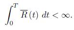
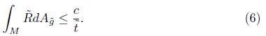
Theorem 1.2. The total scalar curvature for the normalised flow, under the assumption that k g0 ≤ 0, satisfies
So we should expect convergence of the curvature towards zero, and indeed we can prove so assuming some symmetries on the initial data (see Section 4.1).
However, the behavior of the unnormalised flow is quite different: even though the total curvature also goes to zero, the curvature is blowing up (see Section 4).
Theorem 1.3.
If k
g0 < 0 and is locally constant, and the length of the boundary in the normalised flow remains bounded away from 0, then there is constant such that
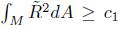 , and, as a consequence, there is a constant
  such that
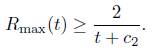
where is the maximum of the scalar curvature at time t.
A natural question to ask is whether there are examples where the length of the boundary remains bounded away from 0. The answer to this question is yes, and indeed we expect that this is always the case. Theorem 3 is proved in Section 4.
Finally, as we said above the convergence towards zero curvature in this case cannot be exponential, in contrast to the case of closed surfaces and of surfaces with totally geodesic boundary. In fact, we prove the following theorem.
Theorem 1.4. Assume that the initial data has the form
satisfies in one of the boundary components (and
 on both), and is locally constant, and that
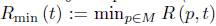 is attained in both components of
 . Then, there is a constant
  such that the normalised flow holds that
Notice that if k g = 0, the convergence is indeed exponential, but once we take kg ≠ 0 in one of the boundary components (and for both components k g ≤ 0), it is not so anymore, as long as the solution to the Ricci flow satisfies the hypothesis of the theorem (explicit examples of initial data so that the solution for the Ricci flow satisfies the hypothesis of the theorem are not difficult to construct). This result is proved in Section 4.
2. Evolution equations and some technical geometric lemmas
In this section, we collect some results to be used in the proofs of our main results.
2.1. Evolution equations
The following evolution equation for the normalised flow is well known (a similar formula for the unnormalised flow holds, see Proposition 2.1 in [3]).
Lemma 2.1. In the normalised flow, the curvature satisfies the boundary value problem
where denotes the outward unit normal with respect to the time evolving metric g (t).
Proof.
The equation in the interior of M is well known (see [4]). The formula for the normal derivative requires some clarification: it comes from the formula for the normal derivative in the case of the unnormalised flow (Proposition 2.1 in [3]) by noticing that this identity is scaling invariant. 
Remark 2.2. Lemma 2.1 has as an immediate consequence that nonnegative scalar curvature is preserved and we leave the proof to the reader. This fact shall be used throughout the paper.
2.2. Geometrical lemmas
Given 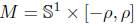 we shall call the curve
  the parallel of latitud s.
Lemma 2.3. Consider a metric of the form
in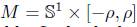 . Assume that there is α > 0 such that
 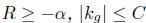 , and let Ls be the length of the parallel of latitude s. Then for any other parallel (including of course any boundary component), we have an estimate
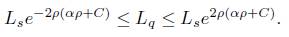
Proof. We prove the upper bound first. First of all, let
where  is the geodesic curvature of the parallel of latitude σ at the point (σ, θ). On the other hand
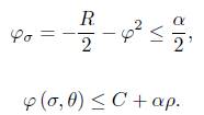
Hence we have
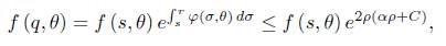
so we obtain the upper bound by integration. The lower bound follows from the fact that in the previous argument, s and q are arbitrary. 
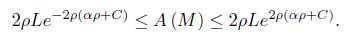
Lemma 2.4. Consider a metric of the form
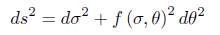
in 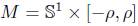 . Assume that there is α > 0 such that
 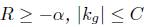 , let L the minimum length of length of the boundary components. Then
Proof. Our point of departure is the following inequality, obtained in the proof of the previous lemma, for  and
and  arbitrary,

From this inequality it follows that
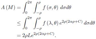
The lower bound is obtained in a similar fashion. 
Remark 2.5. This lemma has as a corollary that whenever the geodesic curvatures of the the boundary components and the diameter of the surface remain bounded, if the length of one boundary component goes to zero, so does the area of the surface. The results of this section will be used to show our longtime existence result for the normalised flow (see next section).
3. Existence for all time
To show that the solution to the normalisation of (1) exists for all time, we follow closely the ideas in [2] and correct some innacuracies found in there. In this section we will assume that the initial metric is of the form
This form of the metric is preserved by both the normalised and the unnor-malised flow.
Our purpose is to show the following theorem, which in turn implies the existence of the normalised flow for all time (see Section 2.1 in [3], beware that the proof given in [5] is not correct).
Theorem 3.1. Assume that the initial data satisfies Rg0 ≥ 0 and kg0 ≤ 0. Then, for any T <  , there exists a constant C (go, T), where R0 is the scalar curvature of the initial metric, such that on (0, T), the scalar curvature of a solution to (1) satisfies
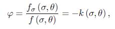
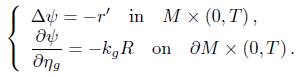
To begin with the proof, first we consider Poisson's equation
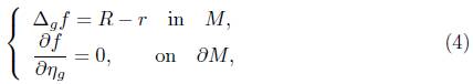
where, as said before, kg is the geodesic curvature of the boundary at time t  and -- denotes the outward unit normal with respect to the metric g (t). We obtain the following result.
Theorem 3.2. There exists a function ψ such that
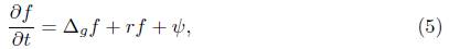
where ψ satisfies an equation
Proof.
The proof is to be found in [2]. However, the value of the normal derivative must be corrected by the arguments given in the proof of Lemma 2.1 above. 
The following lemma will be useful.
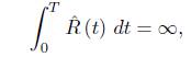
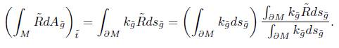
Lemma 3.3. Let r be the average scalar curvature. Then for the normalised flow, and any T <  (so that the normalised flow is defined on [0, T)) we have
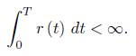
Proof. Notice that for the unnormalised flow the quantity
is nonincreasing under the assumption of nonnegative curvature and  ; it is also scaling invariant, and it corresponds to r in the normalised flow. Hence r is bounded above, and this shows the lemma.
Lemma 3.4. Let  be the value of the scalar curvature when restricted to one of the components of the boundary at time t. Then we have that
Proof. First notice that the conformal factor at any point is given by
so if the conclusion is false, by Lemma 2.4 we must have that the area of the surface approaches 0. Indeed, the diameter remains bounded, since R > 0, and by the previous lemma  for any finite t. This would contradict the fact that the normalised flow keeps the area constant.
We employ now the notation
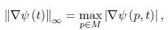
where  represents the norm of
  with respect to g (t). Then we have the following lemma.
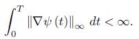
Lemma 3.5.
For any T < we have that
For the proof of this lemma we will use the following elementary result whose proof we leave to the interested reader.
Lemma 3.6. Assume that β 1 and β 2 are continuous positive functions such that
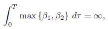
then there is an j = 1, 2 for which
Proof of Lemma 3.5. Notice that by Bochner's formula  is subharmonic,
Hence, by our symmetry assumptions, which imply the same symmetry for ψ, if we let β j·, j = 1, 2, to be - k g R in each of the components of the boundary, then we have
But if
since  remains uniformly bounded away from 0 in at least one boundary component over any finite interval of time (notice that if k
g = 0 there would be nothing to prove, as this case is already considered in [1]), we must also have
remains uniformly bounded away from 0 in at least one boundary component over any finite interval of time (notice that if k
g = 0 there would be nothing to prove, as this case is already considered in [1]), we must also have
where  is the maximum of the scalar curvature when restricted to the boundary, but this contradicts Lemma 3.4.
Now we let
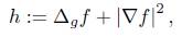
and compute an evolution equation.
Theorem 3.7. h satisfies an evolution equation
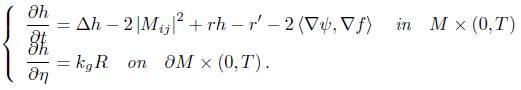
Here  denotes the inner product given by g (t).
The proof of this theorem can be found in [2]. From the previous result we find that h satisfies the differential inequality
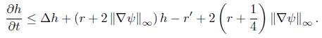
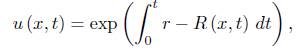
Let
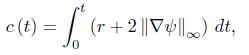
and define
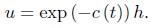
Recall that for any finite T, both  and
and  dt are finite. Then u satisfies the differential inequality.
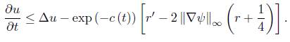
Finally, let
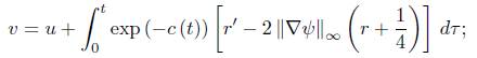
then, since k g ≤ 0 and R ≥ 0, v is easily seen to satisfy
By the maximum principle, v is uniformly bounded on (0, T), and in consequence so is R.
4. Asymptotic behaviour
In this section we remove the assumption of any symmetry. The results we shall present, unless otherwise stated, are valid as long as the initial data has nonnegative curvature. First, we recall a result from [5] (notice that in the statement presented here the hypothesis of symmetry have been removed).
Theorem 4.1. In the unnormalised flow, the total curvature satisfies the estimate
Proof.
As said before, the quantities with a tilde refer to the unnormalised flow (for instance  is the area of the surface with respect to the metric
  ). We start then by calculating as follows:
Writing
by the Gauss-Bonnet theorem, we obtain
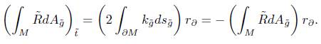
Using that 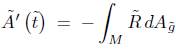 , and integrating the previous identity, we obtain that for some constant c1 > 0 independent of
  ,
,
As we can write 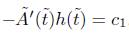 , where
 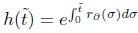 , we proceed as in [5] to obtain
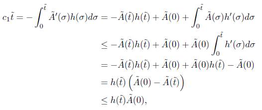
and we arrive at estimate (6). 
The previous theorem has the following consequence for the behavior of the total curvature in the normalised flow.
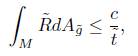
Theorem 4.2. Under normalised Ricci flow, the total scalar curvature satisfies
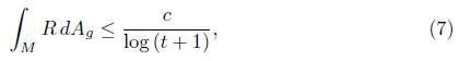
for some positive constant c independent of t.
Proof. From the previous lemma we have that in the unnormalised flow the total scalar curvature satisfies the estimate
for some positive constant c independent of time  . Since under the Ricci flow, as we are assuming Rg ≥ 0, the area
  of the surface is decreasing and its derivative satisfies
  , we can assume, without loss of generality and to simplify the estimates below, that
  . Then we have the inequality
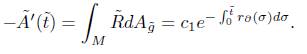
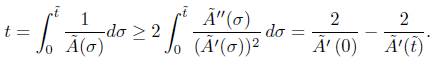
Intregrating with respect to  we obtain
which implies
Now, we integrate the previous expression with respect to time  . This yields
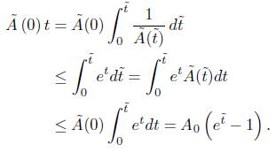
Hence we get that
Since the total scalar curvature is scaling-invariant, i.e
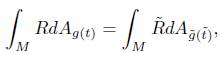
the result follows. 
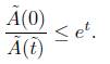
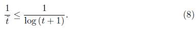
The previous result and its proof have two interesting consequences. The first one is that the unnormalised flow must exist for all time, otherwise inequality (8) would not be valid. On the other hand, we must have that the minimum of the scalar curvature 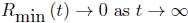 . We state the first of these facts in the following corollary.
Corollary 4.3. If the normalised flow (2) exists for all time, then the unnormalised Ricci flow (1) also exists for all time. As a consequence, if the initial data is of the form
the unnormalised flow exists for all time.
The informed reader must compare this result with the case of closed surfaces of Euler characteristic 0: both the normalised and unnormalised flow coincide, so both exist for all time.
From Corollary 4.3 we can conclude that the curvature in the unnormalised flow (at least when assuming symmetric initial data, see Section 4.1 below) remains bounded on any finite interval of time; but it does not remain uniformly bounded, as the following result shows.
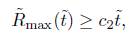
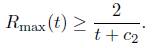
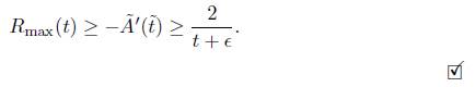
Theorem 4.4. If the length of the boundary in the normalised flow remains bounded below (away from 0), and kg < 0 is locally constant, then there is constant c1 > 0 such that 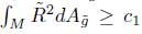 and as a consequence, there is a constant c
2
> 0 such that
and as a consequence, there is a constant c
2
> 0 such that
Proof. If we assume for the normalised Ricci flow that the length of the boundary components are bounded away from 0, then there is a constant C > 0 such that for all t > 0
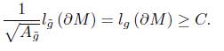
This inequality implies
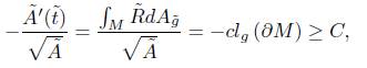
where c < 0 is the minimum of the geodesic curvature of the boundary. On the other hand, by the Cauchy-Schwarz inequality we have
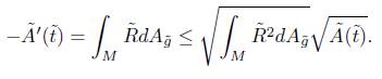
Therefore, we obtain the inequality
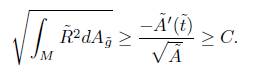
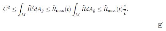
To show that  blows-up in infinite time, we use this lower bound and estimate (6) as follows
One result to be expected in geometric flows is that whenever there is convergence, this convergence is exponential. In our case this is not true; even though the curvature seems to be approaching 0 (at least it does so in an L 1 sense, and in some cases, as shown below, uniformly), it does not do so too fast, and by this we mean exponentially fast, as the following estimate shows.
Theorem 4.5. Assume that the initial data is of the form
satisfies in one of the boundary components (and k
g
≤ 0 on both), and is locally constant, and that Rmin (t) is attained in both components of
in one of the boundary components (and k
g
≤ 0 on both), and is locally constant, and that Rmin (t) is attained in both components of . Then, there is a constant c2 > 0 such that for the normalised flow holds
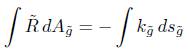
Proof. We let k1 and k2 be the constant values of the geodesic curvature in each connected component of the boundary, and let  and
and  be the lengths of each component. Now notice that, by the Gauss-Bonnet theorem,
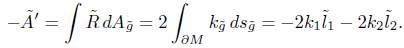
On the other hand
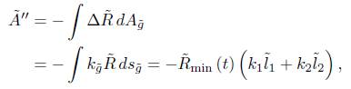
from which we obtain
But
and hence
Then
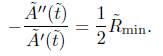
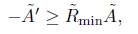
and we can compute
The assumption R
g0 > 0, implies that for an  , so we have
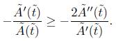
which implies, via the fact that 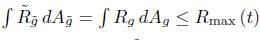 ,
,
We must point out that examples of initial data so that Rmin (t) is attained in both boundary components of M are easy to construct (see [2,5]).
Remark 4.6. Notice that in the proofs of Theorems 4.2 and 4.4 all that is required is that  remains positive on any finite interval [0, T], which is true as long as kg < 0 in any of the connected components of
  (of course, we are also assuming that kg ≤ 0 on both components).
4.1. Assuming more symmetries: refined asymptotic results.
If we assume additional symmetries on the initial metric, we can sharpen our results on the behavior of the curvature. Notice that so far we have been able to prove that the scalar curvature remains bounded over finite time intervals. Let us recall some of the terminology used so far, we write
and we will call  the middle parallel.
Now we shall assume that not only the initial data is of the form
but also that it is symmetric by reflection with respect to the middle parallel. We will assume as well that the scalar curvature Rg
0
≥ 0 is decreasing as we move from the middle parallel towards any of the boundary components. These properties of the initial data are preserved under the Ricci flow as considered in this article (when the solution is at least  ), and we will say in this case that the scalar curvature is decreasing from the middle. Examples where the metric satisfies the properties described above are easy to construct (see Proposition 3 in [5]). The following results shows that under these additional assumptions we can prove that the curvature is uniformly bounded above and even that it approaches 0 as
  .
.
Theorem 4.7. If the scalar curvature of the initial data is decreasing from the middle, then there exists a sequence of times  such that
 .
.
Proof. Notice that being the minimum located at the boundary, there exists a c > 0 such that the length of each boundary component is bounded from below by c for all time. Hence, the diameter of the barrel must remain uniformly bounded by the results of Section 2. On the other hand the length of the middle parallel behaves as
and hence it is decreasing. But the length of the middle parallel must remain bounded away from 0; otherwise, the area of the barrel would go to 0. Hence,  remains uniformly bounded (incidently, notice that the integrand is positive), so for any k > 0 there must exists a tk such that
  . But we have already shown that r
  0 as t
  , and this implies that
Now we prove that the curvature remains uniformly bounded.
Theorem 4.8. The scalar curvature remains uniformly bounded in the normalised flow.
Proof. The maximum of the scalar curvature satisfies
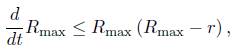
and hence, given any τ, we have that

and we know that 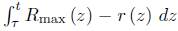 is uniformly bounded, so the result follows.
From the previous two results we can finally conclude:
Corollary 4.9. In the normalised flow  .
.
Proof. Just observe that for any  > 0, there is a t* such that
 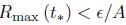 (by Theorem 4.7), where A is a bound on
  , and hence by (9),
Finally, this corollary, by the arguments in Section 2.1 in [3], implies that the solution to the normalised Ricci flow, under the assumption that the initial data has  symmetry, positive scalar curvature and that its curvature is decreasing from the middle, converges smoothly to a metric of zero curvature and totally geodesic boundary.

