


 English (pdf)
 Article in xml format
 Article references
 Send this article by e-mail
 Cited by SciELO
  Cited by Google
  Similars in
SciELO
Similars in
SciELO  Similars in Google
 Permalink
Introduction
The distortion, signal weakening, and the loss of resolution affect the wavelet during propagation, masking the recorded seismograms’ information. Mathematically, the seismic trace results from the convolution of Earth’s reflectivity profile with the signature of energy released by the source (Yilmaz, 2008). Nevertheless, deconvolution is a linear operator that compensates for the distortion of a recorded signal, increases the seismic data bandwidth, and extracts the Earth’s reflectivity. The reflectivity profile requires the highest reliability and resolution possible because it is the capital input of subsequent pre-stack steps of a data processing sequence and seismic inversion procedures. The most used deconvolution in the oil industry is the double inverse of Wiener-Levinson in time WLDI (Robinson and Treitel, 2000) and frequency FDD (Claerbout, 1985). In the case of a free noise seismogram and known stationary minimumphase wavelet, the deterministic deconvolution supplies a highly trustworthy reflectivity. The wavelet is estimable in offshore data but not on onshore one, and in both cases, it is still non-stationary and noise-contained. The free noise assumption is tough to honor due to the impossibility of getting signals utterly free of noise. On the other side, the predictive deconvolution seeks the prediction error representing the reflectivity function. When the prediction distance is one sample, the prediction error filter becomes the optimal zero-lag inverse filter, appropriate in the often fair minimum phase approximation. Even though predictive deconvolution has been a handy tool for several years, it is ineffective under any infringement of the three underlying assumptions. Besides, there is the white spectrum reflectivity assumption. Nevertheless, when the rock layering is periodic, its reflectivity sequence is not random, and the processing flow must resort to alternative methods. Even though the extensive use of statistical procedures, there is no comprehensive response to the three anterior suppositions (Ziolkowski, 1991).
The Homomorphic deconvolution - HOMD (Ulrych, 1971) and the Phase Inversion deconvolution - PID (Lichman and Northwood, 1995) estimate the amplitude spectra of wavelet and reflectivity in the Cepstrum domain where these spectra must not overlap. Both deconvolutions have to fulfill the stationary and the noise-free wavelet assumptions but not the random reflectivity and the minimum phase ones (Arya and Holden, 1978). Crump (1974) designed the Kalman Filter matrixes for deconvolution, and later, Mahalanabis et al. (1983) improved the storage and updating of the matrix by estimating both the smoothed forward and backward prediction residuals of the trace, turning the algorithm computationally more efficient. Despite the above, the high computational cost remains. Recently, Deng et al. (2016) presented a Kalman Filter approach where the reverse wavelet slides over the reflectivity function instead of slides the reverse-reflectivity over the wavelet, as the conventional Kalman approach does. As a result, the number of parameters can diminish until one, and its selection should balance resolution and noise. The Kalman Filter for deconvolution substantially extends the Wiener filtering to accommodate time-varying processes, without supposing assumptions, except noise with a normal distribution of mean zero. In this research, we designed and implemented in Matlab an Extended Kalman Filter to Adaptative deconvolution - EKFD of seismic data based on the approximation of the linear system through the extension of the discrete Kalman Filter (Julier and Uhlmann, 1997). Besides, we implemented in Matlab the deconvolution methods of the double inverse of Wiener-Levinson, Phase Inversion, and Extended Kalman Filter. Finally, the comparison of its outputs allows us to know the impact of the suppositions of deconvolution on the performances of considered methods.
Theory
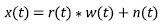
If a wavelet w(t) remains constant during its propagation, the reflected signal will be the superposition of delayed wavelets, with their amplitudes scaled according to the faced reflectivity r(t) along its path and the degree of geometrical divergence. According to the convolution model, a seismic trace x(t) contaminated with noise n(t) is:
 (1)
(1)
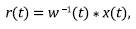
The * symbol represents the convolution operator. The suppositions of the isotropic, horizontal and parallel layered medium, and the plane wavelet that incises normally on the interfaces are necessary to construct the convolutional model. The absence of noise, the known stationary wavelet of minimum phase, and random reflectivity are assumptions required to solve equation 1. The deconvolution attempts to remove the wavelet from the seismic trace to retrieve the earth reflectivity. Under the above restrictions, the Deterministic deconvolution solves equation 1.
 (2)
(2)
w -1 (t) is an inverse such that w -1(t) * w(t) = δ(t) and δ(t) is the Dirac Delta function.
Of course, it is impossible in onshore projects to determine without any uncertainty the wavelet from explosive sources, and vibrators and in offshore from air guns, making unfeasible the deterministic convolution.
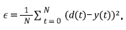
The WLDI is a widely used stochastic approach to solve equation 1 that build an optimal filter by minimizing the square mean error ϵ between the recorded trace y(t) and the signal d(t) desired and supplied by the filter f(t), according to the expression:
 (3)
(3)
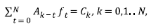
The minimizing condition expressed as ∂ϵ ⁄ (∂ft = 0;∀t = 1⋯N, provides the following set of N coupled equations (Robinson and Treitel, 2000):
 (4)
(4)
Where the vector C
k
represents the cross-correlation between the vectors
 and
and
 , and A
k-t
is the Toeplitz matrix that represents the autocorrelation of
. A recursive approach provides the solution of the equations system 4, i.e., the filter f that extracts the reflectivity. WLDI supposes a random reflectivity that implies that the trace autocorrelation scales the wavelet autocorrelation. In addition to the above, WLDI assumes no-noise, a minimum and stationary phase wavelet, the filter length plus another factor that guarantees the algorithm stability. However, some researchers (Arya and Holden, 1978; Jurkevics and Wiggins, 1984) demonstrated that WLDI is not reliable because of the assumptions’ non-compliance.
, and A
k-t
is the Toeplitz matrix that represents the autocorrelation of
. A recursive approach provides the solution of the equations system 4, i.e., the filter f that extracts the reflectivity. WLDI supposes a random reflectivity that implies that the trace autocorrelation scales the wavelet autocorrelation. In addition to the above, WLDI assumes no-noise, a minimum and stationary phase wavelet, the filter length plus another factor that guarantees the algorithm stability. However, some researchers (Arya and Holden, 1978; Jurkevics and Wiggins, 1984) demonstrated that WLDI is not reliable because of the assumptions’ non-compliance.
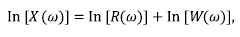
In case of no noise, the Neper logarithm of the Fourier transform of equation 1 becomes:
 (5)
(5)
X(ω), R(ω) and W(ω) are the amplitude spectra of x(t), r(t) and w(t) respectively.
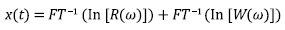
Using equation 5, Ulrych (1971) attempted to separate the R(ω) and W(ω) by converting equation 5 into the time through the inverse Fourier transform:
 (6)
(6)
Since W(ω) is a function smoother than R(ω), they are separable in this denominated Cepstrum domain, but not their phase spectra (Lichman, 1999). A low pass filter retrieves the wavelet contribution, whereas a high pass filter recovers the part of the reflectivity, maximum the separation in case of minimum-phase wavelet. The named HOMD approach requiring neither a random reflectivity nor a minimum phase wavelet assumes that R(ω) and W(ω) do not overlap in the Cepstrum domain (Arya and Holden, 1978). On the other hand, the recovery of the wavelet phase spectrum is not a well-established procedure that depends mainly on the processor (Lichman and Northwood, 1995).
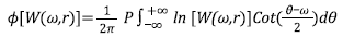
The PID (Lichman and Northwood, 1995) is a homomorphic deconvolution that retrieves the wavelet phase spectrum by using the next Hilbert transform relationship:
 (7)
(7)
In equation 7, P denotes the Cauchy principal value. However, both HOMD and PID cannot separate the spectra wholly in the presence of low-frequency noise or when reflectivity contains low-frequency components.
Kalman Filter
The Kalman Filter (Kalman, 1960) optimally controls and estimates white-noisy linear system models. It achieves the best estimation of a hidden variable immersed in a measurement, based on the information supplied by sensors, control action, and the system’s state at a previous instant. Analytically, the Kalman Filter assumptions are:
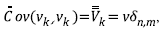
A) The noise measurement V k has a zero mean 〈v k 〉=0 normal distribution and diagonal covariance matrix:
 (8)
(8)
B) The processing noise ω k has a zero mean 〈ω k 〉=0 normal distribution and diagonal covariance matrix:
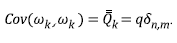 (9)
(9)
C) The measurement and processing noises are independent, i.e. Cov (v k¸ ω k ) = 0.
A variable set characterizes the system in time k and defines the xk state. Equation 10 relates states x
k
, x
k-1
of k , k ̶ 1 instants, where
 is the transition state matrix,
 is the controlling action matrix and u
k
is the control action on the system.
is the controlling action matrix and u
k
is the control action on the system.
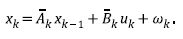 (10)
(10)
Equation 11 relates the x
k
system state with the measurements z
k
in the sensors at instant k through the matrix
 and the random noise v
k
.
and the random noise v
k
.
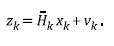 (11)
(11)
In the first phase, the Kalman Filter obtains a first estimate of the current system state
 as from the predecessor corrected state
 using equation 10,
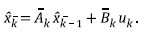 (12)
(12)
Equation 13 relates the covariance matrix for estimated state with the covariance matrix for corrected state , the processing noise covariance matrix given by equation 8, the transition state matrix and its transposed one .
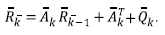 (13)
(13)
The second step calculates the Kalman gain matrix =
 Cov(x
k
¸z
k
) / Cov(z
k
¸z
k
) to diminish uncertainty, expressed in terms of the system matrixes as
Cov(x
k
¸z
k
) / Cov(z
k
¸z
k
) to diminish uncertainty, expressed in terms of the system matrixes as
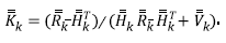 (14)
(14)
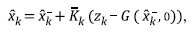
The corrected state
 becomes:
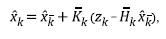 (15)
(15)
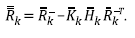
and the corrected state covariance matrix is:
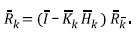 (16)
(16)
Extended Kalman Filter
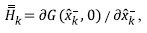
To overcome the fact that non-linear systems do not meet the Kalman assumptions, Julier and Uhlmann (1997) proposed the Extended Kalman Filter approximation. In this approach, equation 13 transforms into:
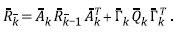 (17)
(17)
Where
 and
and
 are Jacobian matrices of the state transition system constructed as first-order partial derivatives of the state transition equation 10 when ω
k
= 0:
are Jacobian matrices of the state transition system constructed as first-order partial derivatives of the state transition equation 10 when ω
k
= 0:
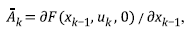 (18)
(18)
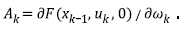 (19)
(19)
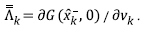
The Kalman Extended Filter gain is now:
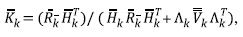 (20)
(20)
 and Λ
k
are Jacobian matrices of the statemeasurements system constructed as first-order partial derivatives of the state transition equation 11 when v
k
= 0:
and Λ
k
are Jacobian matrices of the statemeasurements system constructed as first-order partial derivatives of the state transition equation 11 when v
k
= 0:
 (21)
(21)
 (22)
(22)
The state of the system
 and its covariance matrixes
 are:
are:
 (23)
(23)
 (24)
(24)
The anterior Extended Kalman Filter expressions correspond to the first-order approximation. Their reliability depends strongly on the non-linearity of functions and the assumption of slight variations in each time interval. EKFD approach to deconvolution is essentially a predictive deconvolution that handles time-varying processes (Arya and Holden, 1978).
Methodology
Three different Matlab codes implemented the deconvolutions WLDI, PID, and EKFD. They extracted reflectivity from a synthetic seismogram constructed by convolving a 62 Hz causal Sinc wavelet with a welllog reflectivity. The first tests focused on the impact of the assumptions of the noise in the signal and the reflectivity randomness, and another one on the effect of using non-stationarity wavelet. To evaluate the misfit caused by the noise in the seismic trace WLDI, PID, and EKFD deconvolved synthetic traces with different S/N ratios, equating the standard deviation of whitenoise with the standard deviation of the seismogram.
Measure the effect of randomness in WLDI, PID, and EKFD, they extracted the reflectivity of a seismogram provided by the convolution between wavelet and a non-random reflectivity profile and estimated the misfit between both reflectivities. A final test contemplated synthetic traces built by the convolution with a nonstationary wavelet, counting errors of WLDI, PID, and EKFD during deconvolution. Formerly, Ricker, Sinc, and Damped-Sine wavelets as an inputs model to EKFD allow the estimation of their associated errors. The guiding function chosen is the complete synthetic seismogram, q(n) = σ 3-n and v(m)=σ3-m, with the standard deviation σ and 0 ≤ n,m ≤ 20. In a final step, thirteen transition state functions in EKFD provided output errors that determined their impacts.
In the final step, applying the three algorithms to a real shot gather provided images whose quality measures their performances. The common shot gather has 564 traces with 5 seconds record length with a 1 ms sampling rate. The pre-processing of the shot-gather includes amplitude recovery, refraction statics, and attenuation of the direct wave. The evaluation of the results took into account frequency content, reflector continuity, and time-resolution. Notably, the errors associated with the parameters input to the EKFD comprise the wavelet model, guide function, states transition function, processing noise factor q, and noise measurement factor v, and indicated their selection.
Results and Discussion
Figure 1A shows the causal 60 Hz Sinc wavelet, and Figure 1B shows the well-log reflectivity profile that is 60% random. In contrast, Figure 1C contains the synthetic seismogram supplied by the convolution between the two anterior. Figure 1D depicts the quasinormal distribution of the reflectivity coefficients with 0.0015 mean nearby to zero. The sampling interval is 1 ms for all charts.
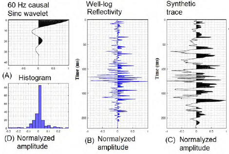
Figure 1 A. Causal Sinc wavelet. B. Well-log reflectivity. C. Synthetic seismogram. D. Distribution of reflectivity amplitudes.
Figure 2A shows the searched reflectivity profile; meanwhile, Figures 2B, 2C, 2D, and 2E contain the reflectivities estimated by KEFD using Spike, Ricker, Sine-damped, and Sinc wavelet, respectively. On the other hand, Figures 2F, 2G, 2H, and 2I depict the errors caused by each anterior wavelet in KEFD. A red box encloses part of the reflectivity profiles to improve the visualization of the result comparison. When using a spike as an input model, the EKFD works like an identity operator because the input (Figure 1C) equals the output (Figure 2B), achieving the highest error shown in Figure 2F. In this extreme case, the use of a spike wavelet makes EKFD out-off-use. On the other extreme, when using a 60 Hz Sinc as an input model, the reflectivity furnished by EKFD in Figure 2E is almost equal to the one observed in the well. In such circumstances, EKFD becomes a deterministic deconvolution with the lowest error contained in Figure 2I. The seismogram in Figure 2C (Ricker), Figure 2D (damped Sine) and Figure 2E (Sinc) look nearly identical to Figure 2A. In these cases, the input models are near similar to the source. Figures 2F, 2G, 2H, and 2I show that the error decreases from 100% to 0.42%. Albeit the input model and the source wavelet seem similar, they do not equal exactly. The evaluation of the parameters of the process noise (q) and the measurement noise (v) indicated a percentage of error below 1% when the ratio q/v < 27 achieved the lowest one errors when q(0)=σ the standard deviation of the trace. When v > q, the results are poor because the measurement noise is higher than the process noise. On the other hand, the minor impact of the 13 transition functions in the EKFD allows us to discard it as a determinant factor. Finally, using the trace as a guide function causes an error comparable to that obtained when not using a guide function, implying the guide function’s unimportant role.
Henceforth, the parameters of the EKFD are a 40 Hz Sine damped function as the input model, length of 150 ms, q equals the standard deviation of the trace and v = q/27.
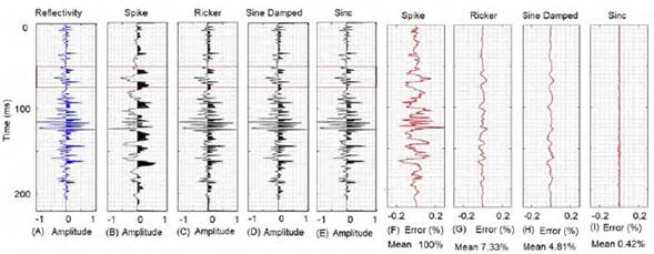
Figure 2 Analysis of input model effect in EKFD performance. A. Well-log reflectivity and estimation using input models, B. Spike, C. Causal Ricker, D. Causal Sine Damped, and E. Causal Sinc. Estimation errors using F. Spike, G. Ricker, H. Sine damped, and I. Sinc wavelet.
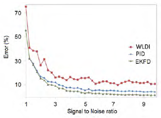
One of deconvolution’s main assumptions is the absence of noise in the trace. To assess it, the application of WLDI, PID, and EKFD to noisy-traces with the signal to noise ratio varying from 1 to 20 provided their respective errors. Figure 3 shows that the estimation errors for all methods decrease when the signal-to-noise ratio increases. As expected, the misfit or is high if the noise is comparable with the signal. PIF and EKF get the most negligible errors achieving values lower than 10% when S/N is over 3.0, while WLDI gets the worst over 10%. But in all situations, EKFD always gets the best performance when the trace contains noise.
The next test evaluated the response of WLDI, PID, and EKFD when they did not meet the randomness assumption. The reflectivity test in Figure 4B indicated that it does not have a normal distribution, verifying its lack of randomness; hence, the trace autocorrelation is not at the same scale that the wavelet autocorrelation. Figure 4A shows the non-random reflectivity used, while Figures 4B, 4C, and 4D exhibit the reflectivities estimated by WLDI, PID, and EKFD, respectively.
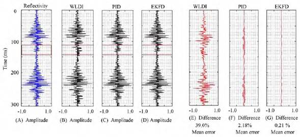
Figure 4 Analysis of the impact of A. no random reflectivity in the output error associated with B. WLDI, C. PID, and D. KFD with different wavelets as input models. Difference between the well-log reflectivity and the estimated ones: E. with WLDI, F. with PID, and G. with EKFD.
Simultaneously, Figures 4F, 4G, 4H, and 4I contain the errors associated with each method. Comparing the WLD I deconvolution and the red box’s trace used, the unfortunate result has an average error of 39.9%, and an evident low-frequency content. On the other hand, PID and EKFD achieve results with minor average errors of 2.18%, and 0.21%, indicating no random trace character.
Finally, to evaluate the impact of a stationary wave assumption, we build a trace decreasing the frequencies of the Sinc wavelet in-depth, starting from 100 Hz up to 20 HZ. Figure 5 shows the predicted reflectivity when the non-stationary wavelet interacts with the well-log reflectivity. Figures 5B, 5C, and 5D show the results of applying WLDI, PID, and EKFD to this trace. In the same picture, Figures 5E, 5F, and 5G contain the errors associated with each method. Figure 5B shows how WLDI cannot extract the rightful reflectivity according to wavelet deepens and pointed out by Figure 5E, where the error increases in depth up to 24.8%. On the contrary, The PID and EKFD recover the reflectivity achieving similar results, Figure 5C and 5D. The corresponding low errors of 4.83% and 3.22% point out the reliability of these two methods. In conclusion, the tests found that WLDI is very sensitive to the stationarity wavelet and to the reflectivity randomness; while, PID and EKFD are insensible to those assumptions. EKFD gets the best results, and although it requires seven input parameters, only the input model and the q/v relation are relevant in the deconvolution and related to the trace.
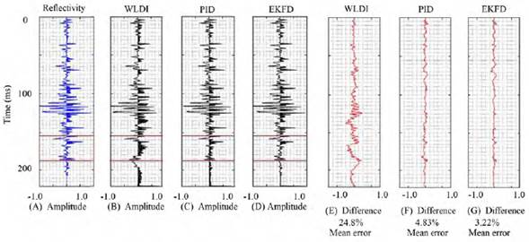
Figure 5 Analysis of the impact of a non-stationary wavelet A. in the output error associated with B. WLDI, C. PID and D. EKFD with different wavelets as input models. Difference between the well-log reflectivity and the estimated ones: E. with WLDI, F. with PID, and G. with EKFD.
In a subsequent analysis (Figure 6), through WLDI, PID, and EKFD estimated the reflectivity profile resulting from the convolution between the nonrandom well-log reflectivity noise-contaminated, and a slightly non-stationary wavelet. Figure 6A shows the reflectivity obtained by WLDI, and focusing on the red box indicates that it does not recover the amplitudes correctly. The misfit occurs throughout the profile (Figure 6D), achieving values in parts of the pattern close to the real ones, with an average error of 10.2%. WLDI is the most used deconvolution in the petroleum industry, with an unreliable result considering that such an outcome is the input to the seismic inversion. Figure 6B contains the reflectivity estimated by the PID. Although it is hard to note considerable differences, Figure 6E shows noticeable discrepancies with the real one at first sight. The average error of 4.08 indicates the PID as a reliable deconvolution.
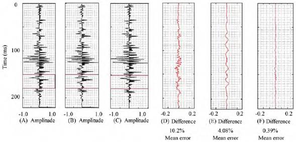
Figure 6 Reflectivity estimated from a trace contaminated with noise and quasi-stationary wave through A. WLDI, B. PID, and C. EKFD. Difference between the well-log reflectivity and the estimated ones by D. WLDI, E. PID, and F. EKFD.
It is worth noting that the absence of low-frequency components in the trace, which favors the PID’s performance. As known, low-frequency components hinder the separation of the signals in the Cepstrum.
Figure 6C shows the reflectivity estimated by EKFD with the best performance achieved. It is supported by the correlation of 0.96 between the real and estimated reflectivity, with a mean error of 0.39% (Figure 6F).
Figure 7A shows part of a common-shot with 564 hydrophones before the deconvolution, with reflectors 1, 2 and 3 to analyze. In Figure 7B, the WLDI deconvolution with a 100 ms time window does not throw optimal results, destroying the lateral continuity of reflectors 1, 2 and 3. Figure 7C contains the common-shot gather after PID, as a result of its application the obtained image looks more focused, maintaining the lateral continuity of the reflectors. Compared with the image achieved by WLDI, the PID image contains higher frequencies in the data. Finally, the result of applying EKFD to the record, in Figure 7D, shows an image with similar coherence and quality provided by PID. The input model for EKFD was a 10 Hz Sinc, corresponding to the dominant frequency of the common-shot gather. The similarity in the quality of the images provided by PID and EKFD is because the marine registry contains a large bandwidth, avoiding the strong restriction of the PID. The zoom to an area of the record marked by the red box reinforces the previous conclusions concerning the three deconvolution methods considered in Figures 8A, 8B, 8C, and 8D. On the other hand, the images provided by PID and EKFD have high-frequency seismic events not generated by spectral whitening, representing registered seismic reflectors. Figure 9 shows the frequency spectra of the shot gathers before and after applying the deconvolutions. Figure 9A shows the amplitude spectrum of the gather without deconvolution. Figures 9B, 9C and 9D show the spectra after applying WLDI, PID and EKFD, with increased high frequency content. Spectra in Figures 9A and 9B have remnants of the shotgun wavelet, characterized by low frequency components of strong energy.
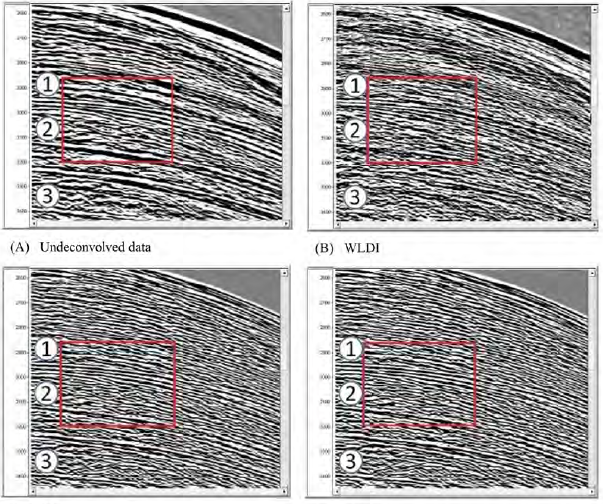
Figure 7 A. Onshore common shot gathers before deconvolution, B. after WLDI, C. after PID and E. EKFD.
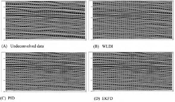
Figure 8 Zoom of the red box area of Figure 7 in A. Onshore common shot gather before deconvolution, B. after WLDI, C. after PID and D. EKFD.
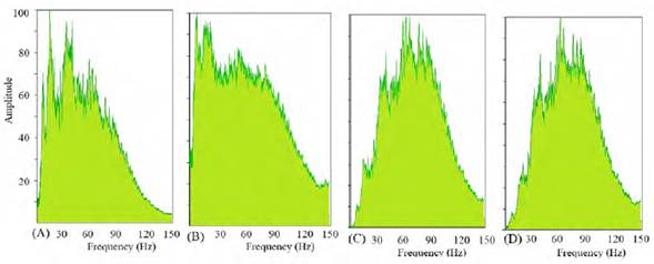
Figure 9 A. Amplitude spectra of shot gather without deconvolution, B with WLDI, C with PID and D with EKFD.
Although WLDI achieves the widest frequency bandwidth, it also increases the power of unreliable components with frequency above 100 Hz. The PID and EKFD spectra look similar with a reliable increase of bandwidth between 20 to 120 Hz. The dominant frequencies in the Amplitude spectra of Figure 9 are consistent with those observed in Figure 8.
Conclusions
The results indicate the lack of reliability of the WLDI to extract the accurate reflectivity from a seismic trace. Such reflectivity is the input to the seismic inversion and puts into doubt its use in deconvolution. Otherwise, EKFD showed a high performance extracting the most accurate reflectivity from seismic traces than the WLDI and the PID. Here, it achieved an error percentage as low as 0.39% and a correlation as high as 0.96 with the pursued well-log reflectivity. The tests with synthetic seismograms demonstrated the EKFD’s robustness to recover the well-log reflectivity. Concerning the deconvolution of offshore seismograms, KFD retrieved the records frequencies and guaranteed the lateral continuity reflectors. Although PID achieved results very close to the EKFD’s, the low-frequency content in the offshore data after processing improved the PID’s output. Into the bargain, EKFD does not require to fulfill the critical assumptions on which deconvolution bases. This paper demonstrates EKFD’s efficacy over WLDI’s and PID’s algorithms. Aversely, EKFD’s performance depends on a suitable input model obtainable from the seismogram through available statistical procedures.

