


 English (pdf)
 Article in xml format
 Article references
 Send this article by e-mail
 Cited by SciELO
  Cited by Google
  Similars in
SciELO
Similars in
SciELO  Similars in Google
 Permalink
Introduction
Reservoir parametrization is an activity in constant evolution that demands significant improvements. Geologists, petro-physicists, and engineers require vast sets of variables to activate models or to establish simulations regarding production rates, reserves, and recovery factors (either in completion or site stimulation). Among these variables, permeability (k), is one of the essential characteristics of the rock that considerably influences the decision-making about field development and impacts the management programs (Helle et al., 2001; Singh, 2005; Kohli and Arora, 2014; Eriavbe and Okene, 2019). Permeability is usually measured from core samples in laboratory tests, being this the most reliable method, however, this is not the solution to parameterize bulky environments since extracting too many cores may be prohibitive (due to financial or physical complications). Semi-empirical formulas are normally used to estimate k values and among the several alternatives, most of them use parameters from well logs (Coates et al., 1991; Saner et al., 1997; Shang et al., 2003; Habibian and Nabi-bidhendi, 2005). A great disadvantage of these formulations is that they work well in a similar medium to the one used for their development (Al Khalifah et al., 2020). Furthermore, the hard mathematical procedures have disadvantages because they demand specific a priori knowledge about the environment and inter-parametric connections. This forces traditional models to limit their performance space within very close limits.
In recent years and following the increase in applications of artificial intelligence (AI) within petroleum engineering, successful approaches have been published using the advantages of AI for the indirect estimation of rock properties. One of the first works that used neural networks to estimate permeability was that of Mohaghegh et al. (1997) . Using as inputs gamma ray, bulk density, and induction resistivity, the authors predict k with sufficiency against selected semi-empirical equations. Other researchers have worked in the same direction (Mohaghegh et al. 1997; Helle et al., 2001; Habibian and Nabi-bidhendi, 2005; Singh, 2005; Maslennikova, 2013; Kohli and Arora, 2014; Al Khalifah et al., 2020) using practically the same inputs than Mohaghegh et al. (1997) with slightly larger training sets. However, due to the nature of the training sets used in these works, the resulting models cannot be applied directly to heterogeneous conditions and their inputs/output ranges are still small-scale.
In this research, the capabilities of Neural Networks NN for estimating k from porosity (ϕ), water and oil saturations (Sw and So) and grain density (GD), obtained from cores, and induction resistivity (ILD), gamma ray (GR) and neutron-porosity (NPHI) from well-logs, are shown. The NN (a multilayer feedforward with supervised backpropagation learning) was trained and tested using 213 core samples from the Morrow and Viola formations in Kansas, United States (KGS, 2020). Due to the size of the database, the ranges of the inputs, and outputs and the heterogeneity of the medium, the neural model presented here is more advantageous and widely applicable than those published so far. Neural evaluations are compared with permeabilities that were estimated using conventional semi-empirical equations (Timur, 1968; Coates and Dumanoir, 1973; Pape et al., 1999), the neural model was also tested in a blind well (well number 8) with outstanding results. It is concluded that the more efficient parametric characterization of the medium, based on k, was achieved with the proposed NN (with the highest correlation values between measured and estimated values).
Neural Networks
Neural Networks are parallel computing processing systems that can estimate any continuous function with arbitrary precision (Goodfellow et al, 2016). The arrangement and operation of the components of a NN attempt to mimic biological learning processes through the association and transformation of input and output data (Singh, 2005). NN are ideal tools for handling substantial amounts of data where the relationship between them is not evident or is too complicated. The structure of a neural network also called architecture, consists of the input layer, one or more hidden layers, and one output layer; each layer is composed of units or neurons. The architecture used in this investigation is a multilayer (various computational layers) and the computations are in a feed-forward manner: successive layers feed into one another in the forward direction from input to output (Aggarwal, 2018) (Figura 1).
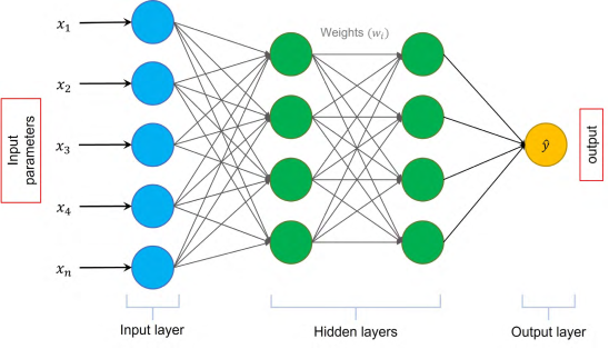
Nodes in the input layer receive external information (inputs) that are processed in the hidden layers to obtain an answer and transmit it to the output layer. This processing might be extremely simple or quite complex, depending on the difficulty of the task. The connections (weights) determine the information flow between hidden nodes (unidirectional or bidirectional) (García-Benítez et al., 2016; Bhattacharya, 2021).
When a NN is trained by a supervised algorithm, learning occurs by changing the weights connecting the neurons, based on the training data containing the examples of input-output pairs. The training data provides feedback on the correctness of the weights in the neural network depending on how well the predicted output for a particular input matches the real output in the training data. Therefore, the training process can be defined as the way a neural network modifies its weights in response to input information. This process is reflected in the modification, destruction, or creation of connections between neurons (Kohli and Arora, 2014; Al Khalifah et al., 2020). The ability to accurately compute functions of unseen inputs by training over a finite set of input-output pairs is referred to as model generalization.
For this research, the backpropagation (BP) algorithm (Rumelhart et al., 1986) was selected to train the NN.
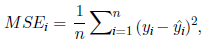
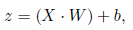
In BP first, a loss function is used to estimate the error between the desired solution and the neural solution. Here, the Mean Squared Error was chosen as the loss function, and it is defined as equation 1:
 (1)
(1)
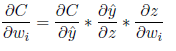
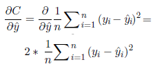
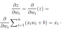
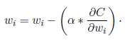
where, MSE i is the Mean Squared Error of the i output, yˆ i is the actual value, yˆ i the predicted value obtained by the neural model and n the number of observations. Then, the best bias, and weights for the NN are determined. This is done through the implementation of gradients (change of the loss function about the bias and weights). Using partial derivation and the chain rule, the gradient of the loss function and the weight wi is calculated (equation 2):
 (2)
(2)
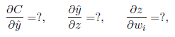
The next three gradients need to be found (equation 3):
 (3)
(3)
where, C is the loss function, ˆy is the predicted value, w i is the weight and z is calculated using equation 4:
 (4)
(4)
where, X is the row vector of the inputs, W is the row vector of the weights and b is the bias.
Starting with the gradient of the loss function concerning the predicted value ( ˆy).
 (5)
(5)
If yˆ=[yˆ 1 ,yˆ 2 ,…,yˆn] and yˆ=[yˆ1,yˆ2,…,yˆ n ] are the row vectors of the actual and the predicted values, the above equation is simplified as:
 (6)
(6)
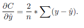
Finding the gradient of the predicted value for z, using the sigmoid activation function as follows:
 (7)
(7)
The gradient of z concerning the weight w i is shown in equation 8:
 (8)
(8)
Therefore:
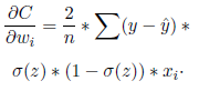 (9)
(9)
Regarding the bias, it is considered to have an input of constant value 1. Hence:
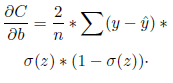 (10)
(10)
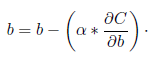
The bias and weights are then updated as shown in equation 11 and equation 12, where the Backpropagation and gradient descent algorithms are repeated until convergence.
 (11)
(11)
 (12)
(12)
Here, the learning rate (α) is a hyperparameter used to control the change in the bias and weights modifying the speed and quality of the learning process. For the interested reader, some selected references are recommended (Coolen, 1998; Cranganu, 2015; Bhattacharya, 2021).
Dataset
The data set was obtained from the online repository of the Kansas Geological Survey, and it is composed of 213 core samples from 8 wells. The core samples used in this work have been sourced from the Morrow and Viola formations (Hugoton Gas Field) and the Forest City Basin (Figure 2).
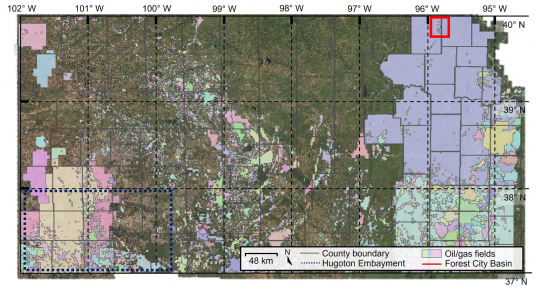
Figure 2 Sampled wells localization, distribution of the sampled formations delimited by a dotted line for the Morrow formation within the Hugoton Embayment and continuous line for the Viola formation within the Forest City Basin.
The lithology from the Morrow formation is composed of shale, limestone, and sandstone, where sandstones are especially abundant (Rascoe and Adler, 1983). The Morrow formation is divided into two units, the lower and the upper unit. The lower Morrow unit is traditionally inferred as offshore shales and shoreline sandstones (Adams, 1964) while the upper unit is constituted by marine shales enclosed by transgressive sequences (Figure 3). A section known as Middle Morrow (Puckette et al., 1996) can also be found, this is a limestone unit with the presence of shales that separates the lower Morrow sandy section from the upper one. Rocks with reservoir functionality are lenticular, ranging from poorly to well classified, with a grain size fluctuating from very fine to coarse, where partially filled cores with calcite, dolomite, quartz, and kaolinite are commonly found.
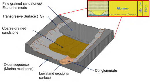
Figure 3 Depositional model and stratigraphic column of the Morrow formation (modified from DeVries, 2006).
Limestone, from the Viola geological group, is found throughout the entire state excluding the northwest, it is composed of fine-grained to coarse limestone and dolomite with a variable amount of shale (Bornemann, 1982). Dolomitized limestone characterizes south-central Kansas, however, toward Forest City and east of the Salina Basin is mostly dolomite. The types of porosity vary, but intergranular, vugular, moldic, and fractures can occur (Caldwel and Boeken, 1985). In southwestern Kansas where it is difficult to discern from Arbucle rocks, the Viola formation ranges from 0 to 20 meters thick on the flanks of the Central Kansas uplift to more than 60 meters in the deepest areas of the Hugoton embayment near the Colorado state line. Based on this lithological description, it is inferred that the sampled arrangements, which constitute the database of this investigation, will present permeabilities in a wide range.
The input properties from core analysis, with the most representative data of in situ conditions, are porosity (ϕ), grain density (GD), water saturation (Sw), and oil saturations (So) while from well logs, induction resistivity (ILD), gamma ray (GR) and neutron-porosity (NPHI). The output is the permeability (k). Table 1 shows a statistical summary of the database used to train and test the neural models.
Table 1 Statistical summary of the properties used in training and testing for the neural models.
| Property | Maximum | Minimum | Mean | Standard deviation | Skewness | Kurtosis |
|---|---|---|---|---|---|---|
| Depth (m) | 1663 | 1080 | 5012.2 | 484.0 | -2.4 | 5.7 |
| ILD (ohm-m) | 495 | 3.1 | 117.5 | 122.3 | 1.3 | 1.1 |
| GR (API) | 148.8 | 14.0 | 44.4 | 28.7 | 2.1 | 4.1 |
| NPHI (frac.) | 0.32 | 0.02 | 0.15 | 0.06 | 0.002 | -0.9 |
| Porosity (%) | 24.1 | 3.0 | 16.6 | 4.4 | -0.82 | 0.4 |
| So (%) | 39.0 | 0.0 | 16.0 | 11.1 | -0.06 | -1.2 |
| Sw (%) | 92.7 | 21.7 | 48.0 | 14.0 | 0.78 | 0.22 |
| GD (g/cc) | 2.85 | 2.65 | 2.68 | 0.05 | 2.0 | 3.2 |
| k (mD) | 2423 | 0.01 | 302.1 | 447.7 | 2.5 | 7.2 |
Results and Discussions
Data pre-processing
Figure 4 shows boxplots of the properties considered inputs in the NN as well as the output (k). This analysis is useful for studying patterns in the data and gaining knowledge about the ranges of the population for each property with which the neural network is intended to be built. The treatment for managing the outliers was conducted by analyzing the k graph. The permeability values around 2300 mD were reviewed to detect errors or to define if it was convenient to keep them in the database. Contradictions between core parameters and these extreme k values were found, so it was decided to separate from the base (5 points, the complete examples). In this new space, a scaling technique was applied to all the input and output variables for each of the ranges shown.
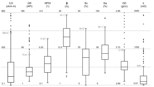
Figure 4 Boxplots for the rock properties included in the database, from left to right: 7 inputs and 1 output (k) (k-permeability, GD-grain density, Sw-water saturation, So-oil saturation, ϕ-porosity, NPHI-neutron-porosity, GR-gamma ray, ILD-induction resistivity).
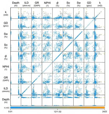
Even with the mentioned preprocessing, the neural task faces a huge challenge, almost impossible for classical modeling methods, since the complexity in the behavior of the property increases when changing to extreme values. Figure 5 shows the matrix plot used to graphically analyze the bivariate relationships between the input properties and permeability.
The neural model construction and its predictions
The whole dataset of 213 core samples was randomly divided into three subsets. The first subset of 60% was used to train the neural network, 18% were separated for testing and the rest, 22%, was used for validation of the NN. To optimize the neural network training process, the K-fold cross validation algorithm was used as a data partitioning strategy to generate a neural model as general as possible, since this algorithm ensures that each instance has served as training and test exactly once. For this neural model 12-folds were used.
The neural architecture was a feedforward multilayer network with backpropagation as a learning algorithm and mean squared error as the loss function. The NN consists of eight inputs (depth, ILD, GR, NPHI, porosity, water saturation, oil saturation, and grain density), one hidden layer and one output (permeability) (Figure 6). One of the critical issues while training a neural network is overfitting, in this research to prevent the model from being incapable to perform well on a new dataset, the convergence curves were monitored to stop the process if the test curve was above the training one, i.e., higher errors while training compared with those obtained for testing. The stopping criterion was the error between measured versus predicted permeabilities. The optimal topology required ~10 thousand epochs to achieve its maximum generalization capacity.
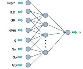
Figure 6 Topology of the neural network for permeability determination, consisting of 8 inputs, one hidden layer, and one output (k-permeability, GD-grain density, Sw-water saturation, So-oil saturation, ϕ-porosity, NPHI-neutron-porosity, GR-gamma ray, ILD-induction resistivity).
The optimum network topology was defined through trial and error, varying the number of hidden neurons, the activation function, and the learning rate (Table 2).
Table 2 Qualification of the different neural models and topologies.
| Neural model | Hidden layers | Hidden neurons | Activation function (hidden layer) | Activation function (output) | Learning rate | R2 training | R2 test |
|---|---|---|---|---|---|---|---|
| 1 | 1 | 270 | Hyperbolic tangent | Hyperbolic tangent | 0.57 | 0.89 | 0.88 |
| 2 | 1 | 50 | Hyperbolic tangent | Sigmoid | 0.50 | 0.90 | 0.86 |
| 3 | 1 | 100 | Sigmoid | Sigmoid | 0.57 | 0.94 | 0.96 |
| 4 | 2 | 175 | Hyperbolic tangent | Sigmoid | 0.45 | 0.91 | 0.90 |
According to the values of R2 in training and test stages, the best topology consisted of 100 hidden nodes with sigmoid as an activation function.
Finally, the NN capabilities were tested using the validation set, which consisted of 48 samples. Since this set is new for the trained neural network it gives an unbiased estimate of the NN skills when comparing or selecting between final models. The topology 8 × 100 × 1 (inputs × hidden nodes × output) is considered the best option (Figure 7).
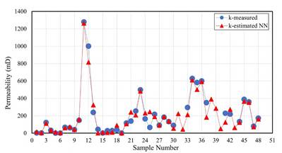
Figure 7 Comparison of measured permeability values against those estimated by the neural network during the validation process.
Prediction results from this topology are shown in Figure 8. According to the fit measurement, it is evident that the prediction behavior is remarkably good.
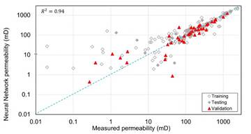
Figure 8 Log-log plot, measured permeability vs estimated permeability by the neural network for training, testing, and validation.
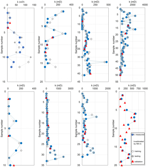
The neural predictions against the permeability measurements for the eight wells in the database, making the distinction between training, test, and validation, are remarkably good (Figure 9), it is important to note that the separated cases for testing and validation were not used to build the model, which means that they are valid and extremely good behavioral tests.
A sensitivity analysis was performed on the NN, and the results of this examination are shown in Figure 10. The uncertainty in the k come from the vagueness in porosity, principally, followed by the water saturation. The hypothesis about the impact of grain density on the model behavior was corroborated. The ambiguity reduction in some tests (NPHI and ILD) has no significant impact on the output, however, after some tests on reduced topologies (eliminating NPHI and ILD), it was concluded that the model cannot be simplified without sacrificing R2.
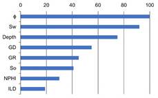
Figure 10 Sensitivity analysis of each input parameter on the neural model (k-permeability, GD-grain density, Sw- water saturation, So-oil saturation, ϕ-porosity, NPHI-neutron-porosity, GR-gamma ray, ILD-induction resistivity).
In Figure 11 cross plots of the relationship between output and every input are shown. As can be seen, the NN estimations are very close to the patterns defined using the lab results. The remarkable neural capabilities are important because these visual representations can be identified (or detected) anomalies that usually are interpreted as the presence of hydrocarbon (or other fluids) and lithologies.
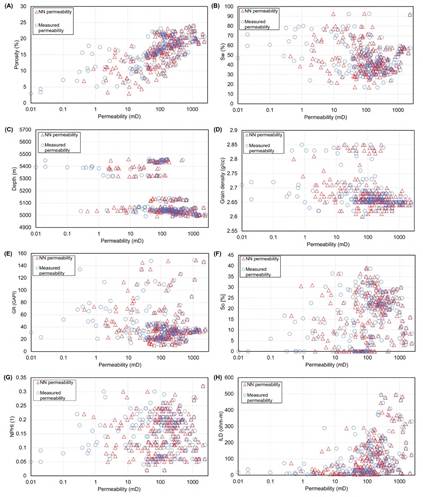
Figure 11 Cross-plots: A. Porosity (%) vs permeability (mD). B. Water saturation (%) vs permeability (mD). C. Depth (m) vs permeability (mD) D. Grain density (g/cc) vs permeability (mD). E. GR (GAPI) vs permeability (mD). F. Oil saturation (%) vs permeability (mD). G. NPHI (1) vs permeability (mD) and H. ILD (ohm-m) vs permeability (mD).
Three conventional equations (Timur, Coates and Pape) were used to estimate permeability and to compare their predictions with the NN estimations. Figure 12 shows that Timur’s model performed the worst, while Coates’ equation was slightly better. Pape’s model remains virtually constant in the requested permeability range; this equation is not sensitive to slight changes in the predictive properties. For the three models and unlike the neural network, the complete range of permeability cannot be estimated correctly, all of them show major dispersion and deviations for permeability values of 300 mD and higher but also for the lowest permeabilities.
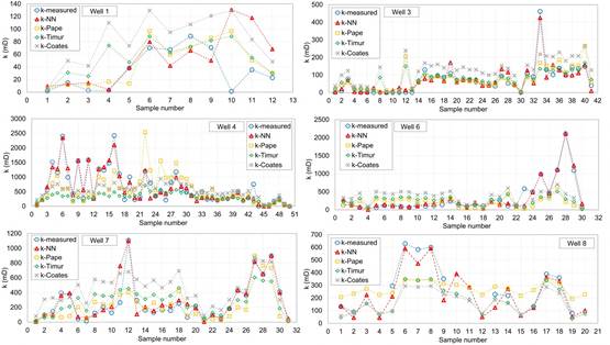
Figure 12 Comparison between the results of the four permeability prediction models (Timur, Coates, Pape, and NN) vs measured permeability for six wells.
Table 3 shows the correlation coefficients obtained by the three conventional models and the NN for the validation set when comparing estimated and measured permeability values.
Table 3 Correlation coefficients (R2) for the predictive models in the validation set.
| Model | R2 validation |
|---|---|
| Pape (1999) | 0.76 |
| Timur (1968) | 0.60 |
| Coates (1974) | 0.46 |
| Proposed neural network | 0.91 |
Conclusions
The NN’s advantageous capabilities for permeability prediction have been shown. Using the neural model here presented, permeabilities can be predicted through easy-to-obtain and economic input parameters. The NN proposed is simple, inexpensive, and meaningful with a remarkable capacity to predict k with high accuracy, despite the complex dependences recognized between properties. The neural model is a powerful alternative to traditional and restrictive statistical tools.
Models like the one presented are very necessary for tunneling (horizontal and vertical), slope stability, foundations, and energy infrastructure design where the intact rock properties are essential. Accurate prediction of k has been an area of interest for rock mechanics for several years, the main advantage of the neural network shown is its dynamic range, that one of the inputs and outputs, it is among the widest of the approximations of its type, maintaining its efficiency in both very low and high values of the output property. This allows it to be used with sufficient confidence in heterogeneous environments or where natural anomalies cannot be ruled out.

