Introduction
The term structure of interest rates (or yield curve, for short) plays a central role in an economy. Current yields have useful information for forecasting future short yields and, potentially, real economy activity, inflation, and other key economic variables (Piazzesi, 2010). Market participants use these forecasts for pricing financial assets, taking investment decisions, and managing financial risks. Central banks use them to inform monetary policy. Consumers use them to make saving and consumption decisions. Thus, superior modeling and forecasting of the yield curve serve policymakers in evaluating past, current, and future economic conditions and help market participants and consumers in taking better financial decisions.
In this paper, we model and forecast the daily yield curve for Colombia using non-arbitrage affine term structure models (ATSMs). The affine term
structure modeling framework dominates the theoretical and empirical literature on term structure models (Piazzesi, 2010). To our knowledge, this is the first study to test the in-sample fit and out-of-sample forecasting capabilities of ATSMs using data for Colombia, which is a necessary step to determine the usefulness of ATSMs.
ATSMs specify the risk-neutral evolution of some unobservable factors responsible for the dynamics of the yield curve by making the yields of different maturities an affine (linear) function of those factors. These models provide a flexible structure for examining the dynamics of zero-coupon bond yields by ruling out arbitrage opportunities. They consistently link the crosssectional and time-series properties of the yield curve (Piazzesi, 2010). The no-arbitrage conditions, in turn, improve the efficiency of the estimates.
Using daily data from 2002 to 2015, we estimate a battery of ATSMs following the estimation methods presented in Ait-Sahalia and Kimmel (2010). We find that a three-factor Gaussian model fits the data and forecasts the daily yield curve for Colombia remarkably well. As Dai and Singleton (2000) point out, Gaussian models are fully flexible regarding the signs and magnitudes of conditional and unconditional correlations of the underlying factors but at the cost of assuming constant conditional variances.1 We find that allowing for conditional heteroscedasticity in the analyzed ATSMs has little effect on the accuracy of the forecasts for our sample data and severely complicates the maximization of the log-likelihood functions. For our daily data, the threefactor ATSM outperforms the one- and two-factor ATSM. The root mean squared errors (RMSE) of in-sample, one, and five day ahead forecasts of average yields are below twenty basis points. This makes the three-factor ATSM especially appealing for pricing financial instruments, taking investment decisions, and managing financial risk. It also offers the possibility of investigating the yield curve dynamics at higher frequencies than those traditionally used in the literature.
56
We show that the factors of the estimated three-factor ATSM closely mimic three widely used empirical proxies for the level, the slope, and the curvature of the yield curve. In particular, the third factor has a strong correlation with an average of the short- and long-run zero coupon yields. The second factor is highly correlated with the slope of the yield curve computed as the difference between ten-year and three-month interest rates. The first factor is highly correlated with an empirical proxy of the curvature computed as twice the four-year yield minus the slope of the yield curve. In addition, principal component analyses produce similar looking level, slope, and curvature factors as those of the three-factor ATSM. Our results are robust to the choice of estimation periods, the use of non-smoothed zero coupon bond yields to estimate the models, and the use of data at lower frequencies (e.g., weekly and monthly).
The article is organized as follows. Section I reviews the previous literature. Section II presents the ATSMs. Section III explains the methodology we use for estimation and forecasts. Section IV describes the data. Section V presents and discusses the main empirical results. The last section concludes.
I. Literature review
Before ATSMs, the dominant framework for explaining the term structure of interest rates was the expectation hypothesis, according to which expected returns are constant over time (Campbell, 1986). The liquidity preference and the preferred habitat theories of the term structure of interest rates can be seen as extensions of the expectation hypothesis, making additional predictions regarding term premiums as a function of the time to maturity of zero coupon bonds. Most tests of the expectation hypothesis reject the existence of constant risk premiums (Campbell & Shiller, 1991; Fama & Bliss, 1987). Thus, modeling time-varying risk premiums is at the heart of ATSMs.
ATSMs date back to the work of Vasicek (1977) and Cox, Ingersoll and Ross (1985). Duffie and Kan (1996) study ATSMs in detail and show how yields for every maturity can be represented as affine functions of some unobserved factors-latent variables. Dai and Singleton (2000) define a canonical representation of ATSMs according to which an Am (N)-ATSM includes N factors, m of which affect the conditional volatility of the other factors. For instance, an A 0(3)-ATSM implies that three homoscedastic latent factors explain the dynamics of the yield curve. Likewise, an A 1(3)-ATSM implies that three latent factors explain the dynamics of the yield curve and that one of the factors determines the conditional volatility of all of them.
Ang and Piazzesi (2003) estimate a discrete Gaussian ATSM incorporating two observable macroeconomic factors: inflation and real activity. Their study finds that macroeconomic factors highly determine the movements of the short and middle ends of the curve, while latent factors are more influential in long yields. They also show, using out-of-sample forecast comparisons, that no-arbitrage cross-equation restrictions make ATSMs more accurate than unrestricted VARs, and that the inclusion of macroeconomic factors further improves their performance. We contribute to the literature in Colombia by estimating a benchmark model without macroeconomic factors as a natural step for future research incorporating them.
Estimating ATSMs is challenging. There exist different methods in the literature (e.g., quasi maximum likelihood, Kalman filtering, simulation, and method of moments, among others). Duan and Simonato (1999) propose a state-space representation of ATSMs and approximate the conditional mean and variance under the assumption that the diffusion process is Gaussian. They estimate the latent factors using the Kalman filter. This allows them to evaluate the likelihood function (quasi likelihood function for non Gaussian models) and estimate the parameters of various ATSMs.
Brandt and He (2006) argue that the quasi maximum likelihood method is skewed for multi-factor models. They present a correction for the quasilikelihood function, which is obtained by simulation and converges to the real likelihood function. This method reduces the skewness and variability of the estimated parameters, but it is computationally intensive.
More recently, Ait-Sahalia and Kimmel (2010) propose a new method to estimate ATSMs. They use closed-form approximations of the log-likelihood functions for the state variables following the methods presented in Ait-Sahalia (2008). They find that their proposed method generates superior parameter estimates.
ATSMs have been used for several purposes. For instance, Singleton and Umantsev (2002) price options on coupon bonds and swaptions using ATSMs. Ho, Huang and Yildirim (2014) propose a method for pricing inflationindexed derivatives based on ATSMs. Duffee (2002) uses ATSMs to analyze the behavior of expected excess returns. Durham (2006) uses ATSMs to model observed and unobserved components of nominal U.S treasury curves and estimate inflation risk premiums.
Another branch of models currently being used for representing the yield curve are the dynamic models derived from the Nelson-Siegel equation, originally proposed by Nelson and Siegel (1987) as a curve-fitting tool. Diebold and Li (2006) re-parametrize the original model to depend on three dynamic factors associated with level, slope, and curvature. They produce forecasts by fitting autoregressive models to these factors and compare them to several other models. While the proposed model performs poorly for short forecast horizons (1 month), results improve as the horizon is enlarged.
These models are further analyzed by Diebold, Rudebusch, Glenn and Aruoba (2006), who include macroeconomic factors in their regressions and allow for correlated dynamic factors. They use variance decompositions to assess the effects of latent and macroeconomic factors on the different ends of the curve, finding a greater influence of the observable factors in short yields.
In a more recent study, Christensen, Diebold and Rudebusch (2011) adjust the dynamic Nelson-Siegel models (both in their independent and correlated factor versions) to be arbitrage free. They derive a model similar to traditional ATSMs, but in which the coefficients of the affine functions that describe yields match the Nelson-Siegel factor loadings. Their results show that the correlated specification has a superior in-sample performance, while the simpler model of uncorrelated factors produces better out-of-sample forecasts. They also suggest that no-arbitrage restrictions improve the forecast accuracy of the models.
This kind of dynamic Nelson-Siegel models has been widely accepted amongst practitioners. It has paralleled the development of ATSMs as dynamic models of the yield curve. The main difference between these two types of models hinges on the no-arbitrage restrictions; but recent studies, such as Christensen et al. (2011), have brought them closer together. A complete review of dynamic Nelson-Siegel models can be found in Diebold and Rudebusch (2013).
For Colombia, most studies model the yield curve focusing on interpolation and curve-fitting of cross-sectional data. The Nelson-Siegel model and cubic splines are the main methodologies used. Few studies use dynamic models, most of them adopting the dynamic Nelson-Siegel framework. Melo-Velandia and Castro-Lancheros (2010) use the methodology in Diebold, Rudebusch, Glenn and Aruoba (2006) to relate monthly yield data for Colombia to macroeconomic factors. They find a strong relation between the model factors (level, slope, and curvature) and the interbank rate, inflation, the GDP gap, and the EMBI. They show, using Granger causality tests, that macroeconomic variables affect the yield curve factors. Maldonado-Castaño, ZapataRueda and Pantoja-Robayo (2014) use the re-parametrization of the NelsonSiegel model presented in Diebold and Li (2006) and apply the Kalman filter to estimate and forecast its factors.
Restrepo-Tobón and Botero-Ramírez (2008) calibrate one-factor arbitragefree interest rate models to daily yield curves in Colombia. Their study concludes that these types of models can closely represent Colombia's term structure of interest rates. To our knowledge, no study has extended these results to multi-factor models and out-of-sample forecasts. We intend to examine these generalizations and forecast capabilities using arbitrage-free ATSMs with daily data for Colombia.
II. Affine term structure models
We denote the yield of a zero-coupon bond with maturity τ by γτ . ATSMs assume that the short-term interest rate is an affine function2 of a state vector X(t) of N underlying factors, which can be observable (macroeconomic variables) or latent (Piazzesi, 2010). Thus,
with δ 0 ∈ R and δ 1 ∈ R N .
The state vector is assumed to follow an affine diffusion process under the risk-neutral measure Q, that is,
where is  an N-dimentional independent brownian motion and
  diagonal matrix with entries
The market price of risk  is also specified in order to obtain the physical dynamics. Following the literature, we assume that Λ(t) = √S(t)λ, where λ is a vector of constants (see Dai & Singleton, 2000). Thus, the state process is also affine under the physical measure P (Duffie & Kan,
1996), that is,
Under this structure, Duffie and Kan (1996) show that the yield for any maturity τ can be obtained as an affine function of the state vector, that is,
The coefficients B(τ) and A(τ) are the solution to the following system of differential equations:
with a(0) = 0, b(0) = ⃗0, A(τ) = −a(τ)/τ, and B(τ) = −b(τ)/τ. These equations come from imposing no-arbitrage restrictions (Duffie & Kan, 1996).
Dai and Singleton (2000) propose a canonical representation in which Σ is an identity matrix. We adopt their notation and representations. As an example, the following equations specify the physical dynamics of three-factor models:
The A 3(3) model:
The A 2(3) model:
The A 1(3) model:
The A 0(3) model:
See Ait-Sahalia and Kimmel (2010) for a full specification of all the models mentioned in this paper.
III. Methodology
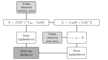
To estimate the models, we follow the technique for maximum likelihood estimation of ATSMs proposed in Ait-Sahalia and Kimmel (2010) and AitSahalia (2008). They approximate the log-likelihood function of ATSMs by a series of highly accurate expansions for the conditional distributions of the state processes. The resulting density expansion from this approach is in closed form. To estimate the parameter vector θ of an Am (N) model, N yields in a panel data of bond yields are assumed to be observed without error. All others yields are assumed to be observed with independent Gaussian errors.
A. The log-likelihood function
For a given parameter vector θ, Equation (6) gives A(τ) and B(τ) for all τ.3 We then form a vector Γ0(θ) (N × 1), whose elements are A(τ), and a matrix Γ(θ) (N × N), whose columns are B(τ), for all τ (maturities) observed without error. The same is done for maturities observed with errors, obtaining Γ e0 (θ) and Γ e (θ).
A vector containing yields observed without errors γne (t) can then be expressed as
using Equation (5). Equation (12) is a linear system with N equations and N unknown variables, which allows us to obtain time series of the values of each state variable in X(t).
Using these estimated state variables, we calculate the estimated yields observed with error using Equation (5).
As in Ait-Sahalia and Kimmel (2010), we denote by pX (∆,x | x 0;θ) the conditional density of X(t+∆) = x given X(t) = x 0 and pγ (δ,γ | γ 0;θ) the transition function of the vector of yields observed without errors. It follows from Equation (12) that
where.  As the conditional density of the state process is not known in closed form in most models, we use the approximations introduced in Ait-Sahalia (2008). The log-likelihood of yields observed without errors at times t
0
,...,tn
with constant time steps of ∆ is then:
Estimates for yields observed with error are obtained using X(t) and
Equation (5). Errors are obtained by comparing the estimates with their ob-b
served values and their log-likelihood is computed using the Gaussian density function. The final log-likelihood function, which we maximize to obtain parameter estimates, is computed by adding the log-likelihood of observation errors with the log-likelihood of yields observed without error. Figure 1 summarizes this process.
B. Optimization procedure
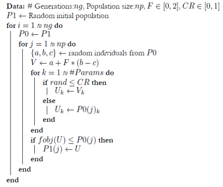
The log-likelihood functions of most ATSMs present multiple local maxima. This makes traditional optimization methods (e.g., gradient based methods) unreliable. In addition, the domain of feasible parameters is restricted for various models. This makes the estimation procedure a difficult task. We turn to heuristic algorithms to maximize the log-likelihood function. In particular, we use the 'differential evolution' heuristic approach (Storn & Price, 1997) given its ability to search for optimal parameter values in a continuous space.
The algorithm works as follows:
Source: authors' elaboration.
Algorithm 1. Differential evolution
Solutions (sets of parameter values) are treated as vectors. We represent the j − th solution of a population P as P(j), and its i − th parameter value as P(j) i . 'Evolution' is recreated by comparing individuals (solutions) from an initial population with new ones and preserving the best. New individuals are generated as linear combinations of individuals from the initial population. Before being compared with the initial individual, they can 'mutate' by changing some of their parameter values with a given probability. This 'evolutionary' process is repeated over numerous generations and the best individual from the last population (according to a given objective function) is taken as the final solution.4
C. Forecasts
ATSMs have mostly been used for monthly and yearly studies of the term structure of interest rates. We intend to evaluate their performance in forecasting the yield curve for Colombia at higher frequencies. Short-horizon forecasts of yield movements can be of help to investors and portfolio managers in building strategies and managing risk. For instance, accurate forecasts could give trading signals or be used to compute measures such as the value at risk of a portfolio.
With the estimated parameters, we find the 'true' state value for the last 'known' date (determined by the horizon) using Equation (5). We then simulate 10,000 state trajectories from this date up to the desired forecast date using Euler's numeric scheme on Equation (4). For each trajectory, we use Equation (5) to obtain yields for all maturities (observed with and without error). We take our forecast value as the mean of the 10,000 simulated points for every maturity.
We also report the simulated 95% confidence intervals for the forecast yields. The limits are obtained by computing the 2.5 and 97.5 percentile points of the 10,000 simulated values for every yield. We repeat this procedure for all days in the validation sample.
IV. Data
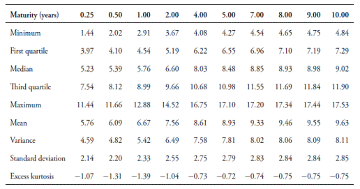
We use daily zero coupon yields estimated using the Nelson-Siegel model obtained from Infoval between January 8 2002 and February 3 2015. The sample includes 3.051 trading days. We use the first 2,000 observations for estimation, reserving the rest for out-of-sample forecasts and validations. Summary statistics for this dataset are presented in Table 1.
We consider maturities of 0.25, 0.5, 1, 2, 4, 5, 7, 8, 9 and 10 years. As pointed out above, for every Am (N) model, we assume that the N yields observed without errors are:
3 months yield for one-factor models.
3 months and 4 years yields for two-factor models.
3 months, 4 years and 10 years yields for three-factor models.
The remaining yields are assumed to be observed with independent Gaussian errors.
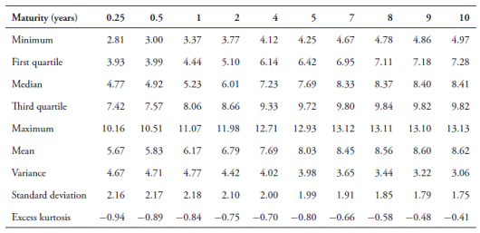
In order to check the robustness of the models, we also work with a data set of bootstrapped zero rates obtained from Bloomberg(r). These zero coupon yields are non-smoothed counterparts of the Nelson-Siegel yields. We use daily observations from April 29 2005 to May 22 2015. The first 1,700 observations are used for estimation. Table 2 presents summary statistics for the bootstrapped yield data set.
V. Empirical results
We estimate nine ATSMs ranging from one to three factors. Following the notation in Dai and Singleton (2000), we consider the following models:
AM (N) with N,M ∈ {1,2,3} and M ≤ N.
The estimation of the models A 2(2), A 1(3), A 2(3) and A 3(3) does not converge using our data. This can be due to the higher complexity that the feasible solution space acquires as conditional volatility is introduced. We tested numerous optimization procedures which either found no feasible solutions or stagnated on initial parameter values. Out of the tested methodologies, differential evolution performed best.
We report results for the models A 0(1), A 1(1), A 0(2), A 1(2) and A 0(3).
A. In-sample Fit
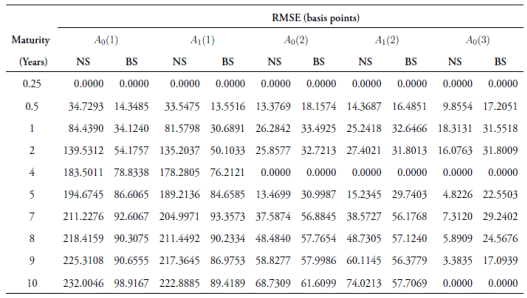
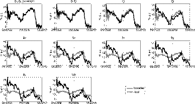
The RMSE for the in-sample fit of each model and maturity is presented in Table 4. The parameter values used for the differential evolution heuristic are presented in Table 3. A plot of the in-sample fit for the model with the lowest RMSE is presented below (all others can be found in Appendix).
Figure 2, when compared with Figures A1-A4 (see the Appendix), depicts how the A 0(3) model outperforms all other models based on its ability to fit the data. Table 4 shows that the in-sample RMSEs for this model are below 18.31 basis points for all maturities. Short and middle-maturity yields obtain higher in-sample errors because of their more platykurtic distributions (Tables 1 and 2). For long-term maturities, the RMSEs are below 7.31 basis points. Thus, based on the RMSE criterion, the A 0(3) model is the best model, which implies that, out of the models taken into account, a threefactor homoscedastic structure best describes the evolution of the yield curve in Colombia.
B. Out-of-sample forecasts
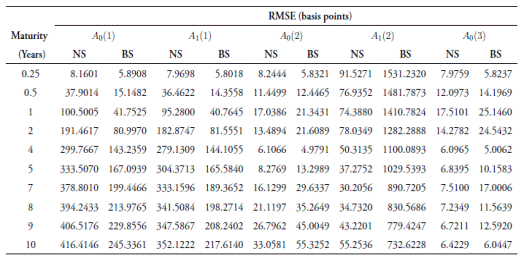
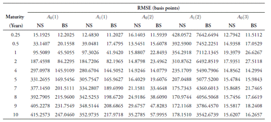
We conduct out-of-sample forecasts for one and five days. Tables 5 and 6 report the RMSEs between the mean forecast (of the 10,000 simulated trajectories) and the observed values. The A 0(3) model outperforms the other models considered in forecasting out-of-sample yields. RMSEs for insample, one- and five-day ahead forecasts are below 20 basis points. Again, shorter yields (0.5, 1 and 2 years) present higher errors, while longer maturities are more stable and easier to forecast.
The A 0(2) model performs marginally better than the A 0(3) in forecasting some of the shorter maturities. However, RMSEs for longer yields (τ > 5) are considerably bigger for the A 0(2).
Apart from the A 0(2) and A 0(3), the models are not good at forecasting the specified maturities. One-factor models fall short when adjusting a high number of yields. In addition, the A 1(2) model presents very large errors, which might be due to complications in the estimation procedure introduced by conditional heteroscedasticity.
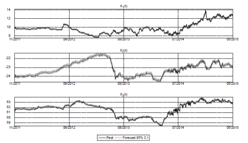
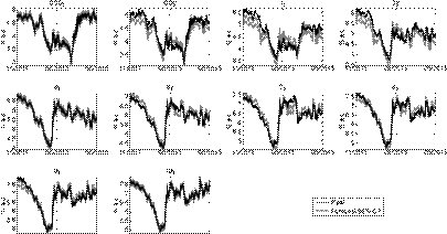
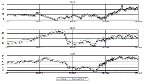
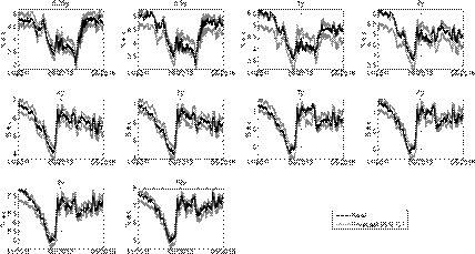
Figures 3-6 show simulated confidence intervals for states and yields forecasts. In line with previous results, short yields have wider confidence intervals and sometimes deviate from them. Longer maturities have narrower intervals and follow them more consistently.
C. Robustness tests
All the results discussed earlier are based on a data set of yields extracted from market data using the Nelson-Siegel method. These yield curves are smoother than what is normally observed in the market. In order to test the robustness of our results, we also use non-smoothed data obtained from zero coupon yields constructed using the bootstrap method, also known as the non-smoothed Fama-Bliss method (Fama & Bliss, 1987), which iteratively builds the discount rate function by computing the forward rates necessary to price successively longer maturity bonds.5
With the bootstrapped yields, our results change little (Tables 4-6). However, both the in- and out-of-sample forecasting errors tend to be slightly higher. The A 0(3) model still outperforms the other models based on inand out-of-sample forecasts for all maturities. However, the A 0(2) model obtains lower errors than the A 0(3) in forecasting shorter maturity yields. Similar to the Nelson-Siegel yields, the A 1(1) model has lower RMSEs than the A 0(1). The big errors in the A 1(2) model also persist.
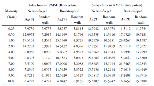
In order to evaluate the A 0(3) model forecast capabilities, we compare its out-of-sample results with a random walk benchmark. We choose this simple model as a benchmark because it has remained hard to beat by models in the literature. For instance, Ang and Piazzesi (2003) find that it outperforms unrestricted vector auto-regressions (VARs), and only manage to slightly beat it (although not for all maturities) using an arbitrage-free model with macroeconomic factors. Duffee (2002) also documents random walks beating ATSMs' forecast capabilities. The one-day and five-day out-of-sample forecast RMSE comparisons are presented in Table 7.
Consistent with the literature, the A 0(3) forecasts are outperformed by random walks. While the shorter end of the curve presents bigger differences in its forecast RMSEs, yields with maturities over four years obtain RMSEs less than two basis points over the random walk benchmark for both one-day and five-day ahead forecasts with the Nelson-Siegel data set.
The higher forecast errors for short yields can be attributed to the lack of macroeconomic factors in our setting. The literature shows macroeconomic factors may play a role in forecasting short and mid-maturity yields (Ang & Piazzesi, 2003).
To further evaluate the performance of the A
0(3) model against a random walk over time and maturity, we analyze the cumulative squared prediction error (CSPE), a metric introduced in Welch and Goyal (2008). The CSPE compares the forecasting performance of a model against a benchmark over time. Calling γi
the measured value of a yield observed at time ,
,  its forecast values by the random walk and A
0(3) models, respectively,
we compute the CSPE as follows:
Table 7 Comparison of out-of-sample forecast RMSE between the A0(3) model and a random walk benchmark
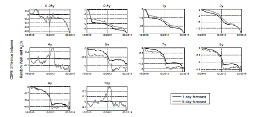
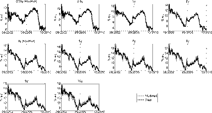
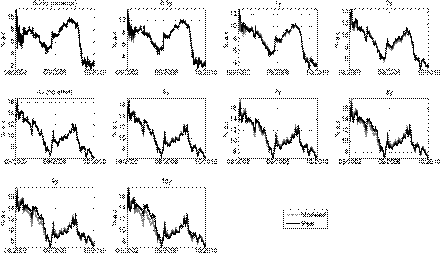
A positive slope in this metric means the A 0(3) model outperforms the random walk over a period of time. We obtain the CSPE for all the maturities over the entire validation sample. Figure 7 presents the CSPE obtained for one-day and five-day forecast horizons using the A 0(3) model estimated with daily observations.
In line with the results from Table 7, all the CSPEs from Figure 7 have a negative value at the end of the validation sample indicating that the random walk model has better accuracy overall. However, several interesting results can be drawn from the behavior of the CSPE metric over time and maturity. For one-day forecasts, CSPEs are very close to zero for the set of maturities which were assumed to be observed without error for the estimation of the model (0.25, 4 and 10 years). This is not the case for the rest of maturities, which have a steady decline in their CSPEs through most of the sample. This marked difference made by the assumption of an observation error in the estimation procedure repeats itself in the five-day forecasts: the A 0(3) is more accurate when forecasting yields observed without error, even surpassing the random walk model for a long period of time around the end of 2012.
When analyzing the effect of maturity on the CSPE, the difference between short and long yields is highlighted again. Yields with maturities of less than four years have a much steeper descend in their CSPE than longer yields. This causes them to have significantly lower final values in both oneday and five-day forecasts. CSPEs for longer yields fall at a much slower rate and even stagnate after 2012, indicating the A 0(3) model and the random walk are similarly accurate from 2013 to 2015.
In order to check the robustness of our results to the frequency of observation, we re-estimate the A 0(3) model using weekly and monthly observations from the Nelson-Siegel dataset. We follow the same estimation and forecast methodologies that were used for daily observations. Table 8 reports the results for weekly data and Table 9 reports the results for monthly ones. Forecasts are obtained with a one-period ahead horizon (one week and one month, respectively).
Table 8 Modeled and forecast RSME for the A0(3) model estimated with weekly observations
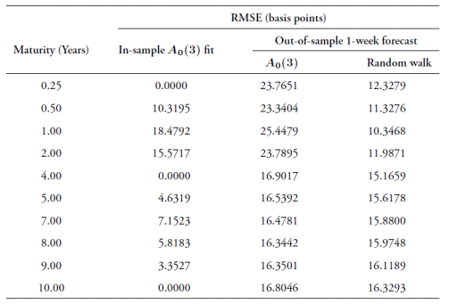
Note: 500 observations were used for estimation, and 124 for forecast validations. Source: authors' elaboration using data from Infovalmer (for the NS set).
Table 9 Modeled and forecast RSME for the A0(3) model estimated with monthly
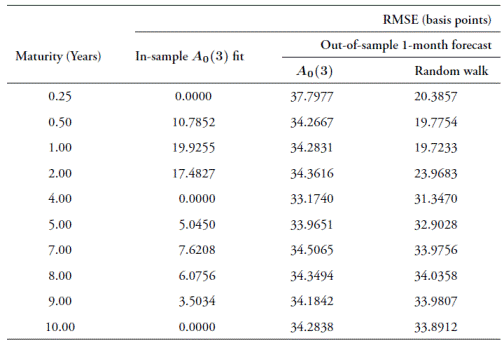
Note: 100 observations were used for estimation, and 49 for forecast validations. Source: authors' elaboration using data from Infovalmer (for the NS set).
Forecast RMSEs are below 26 basis points for the weekly estimations and below 38 basis points for the monthly estimations. As was the case with daily estimations, short term yields have higher errors in the weekly results, but this is not the case with the monthly forecasts.
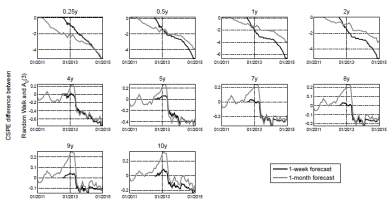
We also compute CSPEs for both weekly and monthly forecasts. These results are presented in Figure 8. The distinction between yields assumed to be observed with and without error during estimation seems to lose relevance at these lower frequencies. For instance, the four-year yield CSPEs resemble those from the five-year yield very closely, which is not the case for daily observations (see Figure 7). Maturity is the differentiating factor in Figure 8, with short yields again having poor performance but yields with maturities over four years showing better accuracy with the A 0(3). One-month forecasts CSPEs also show better behavior than weekly ones, suggesting that lower frequency facilitates forecasting.
Although most studies focus their analyses and forecast tests on lower frequencies, we compare the out-of-sample RMSEs presented here with a few results from the literature as follows:
Duffee (2002) reports RMSEs ranging from 28 to 52 basis points when forecasting U.S. yields with maturities up to 10 years with a three-month forecast horizon using various ATSMs and 'essentially affine' term structure models, which are a more flexible variation of ATSMs.
Ang and Piazzesi (2003) also forecast U.S. yields with maturities up to 5 years and obtain RMSEs ranging from 18 to 30 basis points, making out-of-sample one-month forecasts and updating estimations at every observation. They manage to lower their errors by including macroeconomic factors in their model.
Maldonado-Castaño et al. (2014) use a dynamic Nelson-Siegel model, estimated by Kalman filtering, to produce one-day yield forecasts for the Colombian market. They achieve RMSEs ranging from 21 to 57 basis points for yields with maturities of 3 months, 3 years and 13 years.
Overall, our forecast RMSEs compare well against these results. Our monthly errors are in the range delimited by Duffee (2002), which should be taken as an upper bound considering the longer forecast horizon. One-month RMSEs from Ang and Piazzesi (2003) are lower, but close to our results. Finally, our one-day forecasts achieve lower errors than those reported by Maldonado-Castaño et al. (2014) using Colombian data.
We also compare the modeled latent factors from the A 0(3) model to three empirical proxies for the level, the slope, and the curvature of the yield curve. Following Diebold and Li (2006), we take the following proxies for the empirical factors:
Level: (γ0.25 + γ 4 + γ 10)/3
Slope: γ0.25 − γ10
Curvature: 2γ 4 − γ 10 − γ0.25
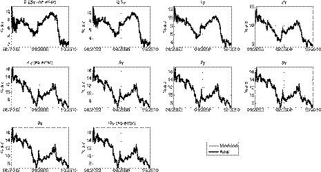
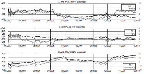
We compare these proxies with the modeled latent factors from the A 0(3) model estimated with the Nelson-Siegel dataset. Results for the non-smoothed yields data set are similar. Table 10 presents correlation coefficients between the estimated A 0(3)-ATSMs latent factors and the empirical proxies for the level, the slope, and the curvature of the yield curve. The three estimated factors have high correlations with the level of the yield curve. The empirical proxies for the slope and the curvature show high correlations with the first and second estimated factors, respectively. Figure 9 depicts these relations.
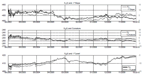
Figure 9 Empirical factor comparison with estimated latent factors for the A0(3) model with the Nelson-Siegel data set
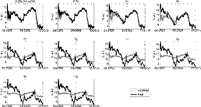
We also compare the three A 0(3) estimated factors with the first three principal components of the yield curve. Table 11 presents their corresponding correlation coefficients. Figure 10 depicts their relations. As with the empirical proxies, there is a strong correlation between the estimated factors and the three first principal components, which together explain close to 96% of the variance of the yield curve.
Table 11 Correlation coefficients between the A0(3) factors and the principal components of the yield data

Conclusions
We estimate five ATSMs using daily data for Colombia. To our knowledge, this is the first paper applying ATSMs to the Colombian bond market. Our main empirical results indicate that a homoscedastic three-factor ATSM fits the data remarkably well. Our results hold under a series of robutsness tests, which include using an alternative data set and data observed at lower frequencies (e.g., weekly and monthly).
We find that the three estimated factors for the ATSM closely mimic the behavior of three empirical proxies for the level, the slope, and the curvature of the yield curve. According to principal components analyses, these estimated factors account for about 96% of the yield curve variance. One- and two-factor ATSMs are unable to describe the behavior of the yield curve in Colombia and should not be used in practice.
Our forecasts have similar errors to those reported in past studies and are close to the random walk benchmark. We encounter larger forecast errors in the short end of the curve, which are highly influenced by macroeconomic factors. Our results can serve as a benchmark for future research in which observable macroeconomic variables could be used. We think this is a natural next step in our research.
We find evidence supporting the assumption of normally distributed measurement errors on some of the yields disturbs forecasts for said maturities at high frequencies. We hypothesize that as our current estimation methodology is only concerned with the distribution of these errors, but not their minimization, other methodologies could yield better forecast results. These errors become less significant as the forecast horizon enlarges possibly due to the increment of variability between observations. This may explain why the existing literature, which focuses on lower frequency analyses, has not yet found this assumption to be problematic.
Therefore, the estimation of ATSMs applying different methodologies from the one used in this paper is also a necessary future development of our research. Because of its complexity, the literature on estimation of ATSMs is growing quickly. It is important to assess whether our results and choice of model hold using novel estimation procedures and to find less computationally intensive routines that can ease the use of ATSMs in the Colombian market.
Our work opens the possibility for future research on the relation between macroeconomic factors and the behavior of the yield curve using ATSMs. A promising area for further work is the identification of empirical macroeconomic factors not spanned by the yield curve and that can potentially be useful in forecasting it.


