


 English (pdf)
 Article in xml format
 Article references
 Send this article by e-mail
 Cited by SciELO
  Cited by Google
  Similars in
SciELO
Similars in
SciELO  Similars in Google
 Permalink
Introduction
Homochirality is a characteristic of living beings related to the chirality of some molecules [1]. At the molecular level, one of the most representative examples of homochirality is the almost exclusive presence of L-amino acids in the proteins that characterise life on Earth. Frank proposed a simple reaction mechanism to explain homochirality's emergence [2]. Subsequently, Kondepudi and Nelson presented a more elaborated version of the same mechanism [3,4]. Many other authors have proposed variations to these models, which are supposed to be better models or, at least, completely different models [5,6]. The analysis of these models gives us insights into the requirements that a chemical network must fulfil to produce the homochirality phenomenon [7]. The first and direct way to perform such an analysis is by computing closed form solutions for the associated systems of differential equations [8]. However, this is only possible for the simplest models. An alternative is the qualitative study provided by linear stability analysis based on spectra of the Jacobian matrixes associated with those systems [9]. Nonetheless, if one must handle large matrixes with non-linear entries, it is difficult to obtain information from them.
Bruce Clarke [10,11] introduced a helpful change of variables that reveal the linearities present in the systems of differential equations: Stoichiometric Network Analysis (SNA). In this paper, we summarise Clarke's work, and we transform it into an algorithm implemented in a computer programme: Listanalchem second algorithm [12]. The results obtained with this algorithm were verified using numerical simulations (time series and bifurcation diagrams) [13-15]. Those simulations were performed using the Chemkinlator computer programme [16]. The correctness of the computed results is remarkable.
We use the aforementioned tools to analyse some of the most representative stoichiometric networks (chemical models or chemical mechanisms) proposed to explain the origin of biological homochirality, including three of the most recent models presented in the literature. We begin our study with the first and most straightforward mechanism, the one proposed by Frank in 1953. This iconic model is tuned in order to obtain models that are consistent with chemical kinetics and the most basic thermodynamic principles. Thus, in this way, we obtain new models that are tested using our analytical tools. We also used the aforementioned tools to analyse other representative models found in the related literature [5,17,18]. These include three recent models, as well as a reaction mechanism proposed by Trapp and co-workers [19]. This latter mechanism is intended to model Soai's reaction [20]; which is, to date, the single experimental reaction that exhibits asymmetric autocatalysis. The model of Trapp et al. seems to be the only proposal that correctly describes Soai's reaction. This assertion is based on a detailed kinetic analysis and reaction modelling corroborating the formation of hemiacetals as the reactive species in Soai's asymmetric autocatalysis.
The result of the total analysis in this work is a set of general characteristics that must be exhibited by a thermodynamic and kinetic consistent model that can produce homochirality.
Materials and methods
Algorithmic analysis of non-linear chemical systems
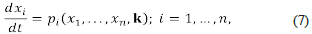
Suppose we have a chemical system constituted by chemical species and chemical reactions, its dynamics is driven by a system of differential equations such as:
where the variables x 1 ,…,x n represent the concentrations of the n chemical species, expressed in a convenient and consistent system of units. The symbol k represents the r-dimensional vector of reaction rate constants that occur in the definition of the functions f i ,...f n . If there exists i≤n such that f i is a non-linear function, for example, a polynomial on the variables x 1 ,...,x n we say that the above system is an autonomous system of non-linear differential equations (a non-linear system, for short). The solutions of those (non-linear) systems describe the dynamics of the concentrations of the species of interest, and the reaction rate constants should be considered variable parameters ranging over an (small) interval of the positive reals. The reader must consider the fact that the value of most reaction rate constants is not known.
Most non-linear systems cannot be solved by analytical means. Hence, the analysis must be a qualitative one based on the linear stability of the steady states [9,21].
Definition 1. We say that (a, k o) ∈ ℝn × ℝr is a steady-state, if and only if, the following equalities hold.

Notice that if a system is driven to the state x1=a1,…,xn=an, under the well-controlled conditions represented by k0, then nothing occurs; the system is stuck at a fixed point of its dynamics. In real life, steady states are reached because of friction, dissipation, or entropy growth. However, we see dynamics all the time. This happens because physical systems are continuously perturbed by external noise, and hence most of the dynamics that we see correspond to dynamics that occur when steady states are perturbed. Thus, it makes sense to study the dynamics that could occur when one perturbates the steady states of the system under study.
The qualitative analysis of non-linear systems studies the dynamics that occur near the steady states. Steady states can be either stable or unstable. The idea is that all the exciting dynamics occur near unstable states. Therefore, it becomes essential to develop mathematical and algorithmic tools for the detection of unstable states. The aforesaid problem, called stability analysis, can be reduced to matrix analysis.
Let (a, ko ) be a steady-state, the Jacobian matrix at state (a, ko ) is the matrix
It has been known, for a long time, that the stability (instability) properties of a state (a, k0 ) can be deduced from the eigenvalues of Ja, ko [9].
Definition 2. Let (a, k 0 ) be a steady-state and let λ 1 ,…, λ n be the eigenvalues of J a,k0. We say that (a, k 0 ) is stable, if and only if, for all i ≤ n the inequality Re (λ i ) < 0 holds, where Re (λ i ) denotes the real part of λ i . On the other hand, we say that (a, k 0 ) is unstable, if and only if, there exists i such that Re (λ i ) < 0, and for all i it occurs that Re (λ i ) ≠ 0
Remark 1. We say that a matrix is a full rank matrix if and only if the set of rows and the set of columns are linearly independent. Notice that the Jacobian matrixes of the stable and unstable states are full rank.
Thus, the stability analysis of the system
is reduced to the analysis of the set

Polynomial Systems. We say that the non-linear system
is a polynomial system, if and only if, for all i ≤n the function f i is a polynomial over the variables x 1 ,.,x n . Suppose that we must analyse a polynomial system
and suppose that we know that the parameters range over the small interval Ω. Let J :ℝ n × Ω r→ℝ be the function

Observe that function J is a polynomial over the variables x1,…, x n , λ, k 1 ,…, kr . Moreover, the set of steady states of the dynamical system is the zero set of the system of polynomial equations given by

This means that the stability analysis of polynomial systems reduces to the analysis of a polynomial function defined over an algebraic variety. Computational algebraic geometry provides us with the algorithmic tools necessary for the stability analysis of polynomial systems.
Unfortunately, most of the aforementioned algorithms are inefficient, and the analysis becomes unfeasible for moderately large values of „ [22]. This fact indicates that it is worth looking for mathematical tools that could reduce the dimensionality of the algebraic objects under study. Stoichiometric Network Analysis (SNA) allows us to reduce the degree of those algebraic objects.
Basic Concepts of Chemical Networks
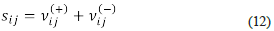
A chemical reaction over the chemical species X 1 ,...,X n is an expression analogous to

where ν 1 ,…,ν n are small integers (some of which could be equal to zero) that are negative ν (-) for the reactants and positive ν (+) for the products. The above expression indicates that the mixture of | ν 1 (-) | units of X 1, …, and | ν n (-) | units of X n gives place to ν 1 (+) units of X 1, …, and ν n (+) units of X n .
A chemical network over the species {X1,...,X n } is a set of chemical reactions, say {R 1 ,...,R r }, over this set of species. Let Ω = [(X 1,..., X n), (R 1,..., R r )] be a chemical network, where R j is the reaction

The network Ω can be encoded into the stoichiometric matrix S Ω , that is given by
The entries of the above matrix are called the net stoichiometric coefficients. These coefficients can be used to determine the number of units of species X i that remain after the occurrence of the reaction R j . Observe that the rows of S Ω correspond to the species and the columns to the reactions.
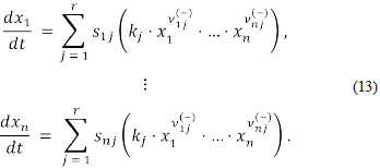
It happens that chemical reactions have different rate constants. Let (k 1 ,..., k r ) be a vector of rate constants and suppose that under some given conditions, these are the rate constants of the reactions R 1,..., R r. Then, the law of mass action [23] determines that the dynamics of the network, under those specific conditions, is governed by the polynomial system:
The work of Clarke: Stoichiometric Network Analysis (SNA)
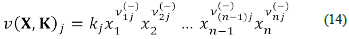
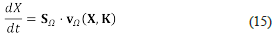
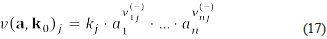
Let Ω = [(X 1,..., X n ), (R 1,..., R r )] be a chemical network. The velocity function of Ω is the function v (X, K): ℝ+ n ×ℝ+ r →ℝ+ r , defined by:
Clarke [10,11] established that the network kinetic equation can be written as
Notice that we are not using the matrix S Ω to linearize the system, we are using it to write the polynomial system in matrix form. Good notations can provide insight: Clarke's matrix form suggests that one can perform the stability analysis in the velocities space instead of in the concentrations space. It happens that switching to the velocities space can reduce the dimensionality of some networks. Moreover, this yields a novel factorisation of the Jacobian matrix, which was (apparently) discovered by Clarke [10], and which is heavily used in SNA. One crucial element of this factorisation is the denominated matrix of extreme currents, Ea. The meaning and implications of this matrix have been used to obtain insights regarding the behaviour of several models proposed for explaining the origin of homochirality from the point of view of spontaneous mirror symmetry breaking (SMSB) [24] and entropy production [25]. Vuk Radojkovic and Igor Schreiber have also proposed a method, based on SNA and constrained linear optimisation, to estimate rate coefficients and steady-state concentrations of classical chemical oscillators [26]. We will not discuss such topics; instead, we will develop algorithmic methods that can be used to compute the parameter values that can produce homochirality in a given network model. That is the focus of the following paragraphs.
Clarke's Factorisation
Clarke's work is heavily based on a factorisation which can help us to simplify the stability analysis of various large chemical mechanisms. This factorisation allows us to reduce the degree of the polynomials that occur in the dynamic equations. We will present this factorisation in two forms.
The first form of Clarke's factorisation. The matrix of orders of reaction (also called the kinetic matrix) is the matrix
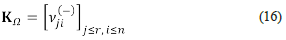
Observe that the rows of K Ω , in contrast with the rows of S Ω , correspond to the reactions (while the columns correspond to the species). As we will see, the kinetic matrix is a key ingredient of Clarke's factorisation. Let us select a steady-state (a, k0) and let us say that this state is our reference state. The state (a, k0) determines a velocity vector VΩ=(vi,...,Vr), which is given by
We have, due to the steady-state conditions, that

and this means that the physical velocity determined by the steady-state (a, k0) belongs to the kernel of S Ω .
Now, suppose that for all i≤n, the inequality a
i
>0 holds. Then, we use the symbol h to denote the vector
 . SNA is based on the following theorem [27], which corresponds to a factorisation of the Jacobian matrix.
Theorem 1. Let Ja,kc be the Jacobian matrix of a system at the steady-state (a, Ko), we have that
The second form of Clarke's factorisation. Physical velocities must satisfy the constraint v(X, K) i ≥ 0. Moreover, at a steady-state (a, k 0 ), the physical velocities must satisfy a further constraint, given by the equation

Solutions to the above two constraints are called currents. The set of all currents is equal to

and it contains the set of physical velocities that can occur at steady states. Notice that the dimension of Cq, that we denote with the symbol c, satisfies the inequality

where d = dim (S Ω ) is the dimension of S Ω , which is the number of linearly independent rows (columns) of S Ω while r is the total number of reactions in the chemical network Ω. If d is big enough, the size of C Ω could be small, and this could help us to ease the analysis. Unfortunately, this dimensionality reduction does not always occur, and it strongly depends on the model (the number of reactions and its stoichiometric matrix). In many cases, the dimension of C Ω is enormous: the inequality c ≧ r - d is just a lower bound. Then, it could happen that the problem becomes one of larger dimension when switching from the concentration to the velocities space.
Note that C Ω is a convex cone, (called the current cone). Also note that C Ω is polyhedral. The current polytope is equal to

Π Ω is a polytope in the geometrical sense, and this means that it is the convex hull of a finite set that we call the set of nodes of this polytope.
Remark 2. Given a finite set of linear inequalities and linear equalities defining a polytope Π, the set of nodes of Π can be computed by algorithmic means.
Thus, given a network Ω, one can effectively associate to Ω a matrix E Ω * such that the columns of E Ω * are the non-zero nodes of Π Ω . The matrix E Ω * is a rational matrix, and it can be scaled to obtain an integer matrix E Ω . The matrix E Ω is called the matrix of extreme currents, and their columns are called extreme currents (they are the extreme rays of the current cone).
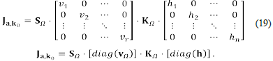
Now, let Ω = [(X 1,..., X n ),(R 1,..., R r )] be a network. According to the first form of Clarke’s factorisation, we can write the Jacobian matrix at (a, k 0 ) as Ja, k 0 = S Ω ⋅ [diag (v Ω )] ⋅ K Ω ⋅ [diag(h)].
Recall that v Ω is a current. It means that v Ω is a positive linear combination of extreme currents; hence it can be written as

for some vector j ∈ ℝs +. Let e ij be the ij -th entry of the matrix E Ω . We have that for all i ≤ r the equality
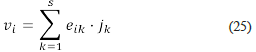
holds.
Let diag (E Ω ⋅ j) be the matrix
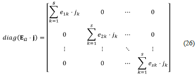
then, we have that

The above factorisation of Ja, k0 corresponds to the second and final form of Clarke's factorisation.
Implications of Stoichiometric Network Analysis (SNA): Reduction to Convex Parameters
The matrix
is a scaling matrix with non-negative entries, and hence it does not influence the signature of the eigenvalues of J a, k0. Thus, we can focus on the matrix V Ω = S Ω ⋅ diag (E Ω ⋅ j) K Ω . Note that S Ω and K Ω are constant (numerical) matrixes that do not depend on our reference state. It is also the case with the matrix EΩ . Then, we can forget the reference state (a,k 0 ). Also, we can see that the entries of diag (E Ω ⋅ j) are linear functions that depend on the convex parameters j 1 ,…, j s . In that case, we can forget the numerical values of j 1 ,…, j s that allowed us to express the velocity VΩ as a convex combination of extreme currents, and we can consider them as the new parameters related to the nonlinearities in concentrations (mass action law) but without their exponents or cross-products.
We use the symbol V Ω to denote the non-numerical (symbolic) matrix

called the current matrix, and which is the matrix that we want to analyse. Note that the current matrix encodes the Jacobian matrixes of all the steady states, and its entries are linear polynomials over the variables j i ,..., j s . Observe that we obtain an important dimensionality reduction by using SNA: the degree of the polynomial entries of Vq matrix is one. Notice that this was possible due to the factorisation of the Jacobian matrix.
The aforementioned reduction can become useless if the number of parameters grows considerably. Note that we are using s parameters, the parameters j 1 ,…, j s , where s is equal to the number of extreme currents (extreme rays of the current cone). We cannot compute, in advance, the exact value of the number of extreme currents that we denote with the symbol #EC Ω but we have that
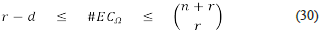
Note that the number of extreme currents can be so huge that the analysis becomes impractical or at least very demanding. Remember that we want to analyse the set

which is a parameterised set of „*„ matrixes that are initially given through „+r parameters. SNA allows us to encode this set into a symbolic „*„ matrix that is given by s parameters.
Computing instability regions
Let Ω be a chemical network. We want to introduce an algorithm that can compute an approximation to the set of unstable steady states of Ω. Let (a, k 0) be a steady-state and let J (a, k 0) be the Jacobian matrix at (a, k 0). If all the eigenvalues of J (a, k 0 ) have a strictly negative real part; then the system is stable. Thus, we are interested in computing the set

Suppose that the characteristic polynomial of J (a,k0) is equal to
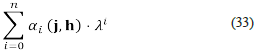
Each one of the terms αi (j, h) is a polynomial expression over the parameters j and h. The coefficient α i (j, h) is equal to the sum of all diagonal minors of J (a, k 0) of order i [28]. On that account, the coefficient α i (j, h) is equal to the sum of all diagonal minors of V Ω of dimension i×i multiplied by the corresponding sets of reciprocal concentrations. Note that parameters j and h are non-negative, therefore any negative term in the characteristic polynomial of J (a, k 0) implies the existence of a diagonal minor of V Ω of order i, whose polynomial expression contains a monomial preceded by a minus sign. We say that a such minor of V Ω is a source of instability. The detection of all the minors that are sources of instability (unstable minors) can be carried out using symbolic algebra [29, 30].
Note that each diagonal minor is determined by a set I ⊂ {1, ..., n}. Let V Ω I ,…,V Ω I be the unstable minors; we say that V Ω I ” is an essential source of instability (essential minor), if and only if, for all i≠m the set I m is not a superset of I i . Each essential minor V Ω I ” determines a polynomial, its determinant, which can be written as

where A m is the set of indices for which a 1 m < 0, and B m is the set of indices for which a i m ≧ 0. We have that set V Q I” < 0 if and only if, the inequality
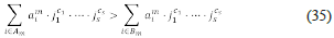
holds. The above polynomial inequality is the instability condition for minor V Ω I m .. We use the symbol Ci, q to denote the latter inequality, and we use the symbol D¡, Q to denote the set

Given J0 ∈ ℝ+ s , it encodes a chemical velocity vΩ-j0. Thus, if we compute J0 ∈ ℝ+ s such that the inequality C I, Ω holds for j0 then there must exist at least one steady-state (a, k0) whose velocity is equal to vΩ-j0. The above facts indicate that the computation of ⋃ I D I, Ω can be of help in the analysis of network Ω. Moreover, the sets D I,Ω are semialgebraic, and semialgebraic sets behave very well from an algorithmic point of view: they can be tested and sampled by algorithmic means [31].
We will present an algorithm derived from the above facts, which can be used in the stability analysis of reaction networks, particularly in this work, those related to SMSB [32]. The algorithm is intended to search for reaction rate constants that are good candidates for encoding unstable steady states. These calculations are implemented as the second algorithm of the Lista„alchem computer programme [12]. The algorithm works as follows:
Define the model, Ω, to be analysed in terms of its species X, and reactions R. If the model has only two species, they are the enantiomers. If there are more than two species, the first two defined in the species list must be the enantiomers. If there are more than two pairs of enantiomers, they must be defined explicitly, and the sixth Lista„alchem algorithm must be used [33] (this will not be discussed here).
Compute S Ω , and extend S Ω . The matrix S Ω is extended with rows that code the duality relation between reactions. This operation decreases the size of the E Ω matrix and the running time of the entire algorithm, enabling it to analyse large mechanisms (networks), something that is usually not possible when matrix S Ω is not extended. This important fact can be tested using Lista„alchem, matrix Sq and its extended version.
Compute K Ω , v Ω , E Ω , diag (E Ω ∙ j) and Vq. In this work, matrix EQ is calculated based either on a previously reported algorithm [29], or on the code of COPASI software [34], both modified to work with singular matrixes.
Compute all the unstable minors of V Ω . In our computer programme, the maximum size of the essential minors is limited to five to avoid long computations. If U 1 D 1 ,q is empty, there are no unstable minors, and the programme finishes, otherwise it goes to the next step.
Compute the system of inequalities and equalities that must be satisfied.
Compute the intervals where the above system of inequalities and equalities are satisfied. If the inequalities are linear, the solutions are found. Otherwise, a heuristic approach is taken to linearise the inequalities. Finding the intervals where the system of inequalities and equalities are satisfied is not an easy task because of the nonlinearities [31]. In our computer programme, the solutions of linear systems are found using Reduce [35], which cannot solve non-linear systems. We use a heuristic and naive procedure that turns the non-linear inequalities into linear ones. The procedure finds, iteratively, the most common j's in the non-linear system and replaces them with positive random values, repeating this operation until the system becomes linear. The selected values may not produce a solvable linear system, but if they do, we can check for the intervals at which they are satisfied with the help of Reduce [35]. If the procedure fails to produce a solvable linear system, the set of values can be re-sampled as many times as desired. This step aims to obtain a set of intervals where the system of inequalities and equalities is satisfied.
Sampling: compute one element of the solution set of the linearised system obtained in the previous step. Random values, generated inside the ranges where the linear system is satisfied, are assigned to j 1 ,…, j k. .
Given the values computed in step 7, compute the corresponding reaction rate constants k 1 ,..., k r , using the relation v Ω = E Ω ∙ j. Convenient values are assigned to the concentrations when necessary.
Test the results by numerical simulations using the respective differential equations and including bifurcation diagrams. In this work, this is carried out using our software called Chemkinlator [ 16].
Concerning steps 4 and 7, some remarks are in order. It is true that given the semialgebraic definition of Ui D i , Ω , it is possible to check by algorithmic means if the latter set is non-empty, and it is also true that one can compute points within U i D i , Ω (provided it is non-empty). But it also happens that the set Ui D i , q could be infinite, and it becomes infinite for most of the chemical networks that one would care to analyse with those tools. Note that, in those cases, the finite samples that we compute can be non-representative. We can reduce the set of target states using chemical-based heuristics or physical constraints, such as solubility or diffusion-controlled rate constants [36]. However, the approach in this work is to sample the instability region, make simulations with that set of rate constants, and then expand the region of analysis through the construction of bifurcation diagrams (step 9 of the algorithm). In this way, we explore the hyperspace region around the unstable points that are computed by the sampling process.
Results and discussion
The reaction networks discussed below can be found in the folder "models" of Listanalchem as "*.py" files. The corresponding name files can be found aside from the titles of the subsequent sections, where we analyse different network models of biological homochirality. Also, the respective plots, equivalent to figures 1 and 2, can be obtained from the data given by Listanalchem, second algorithm (SNA), and Chemkinlator, the two computer programmes used here to obtain the results discussed below.
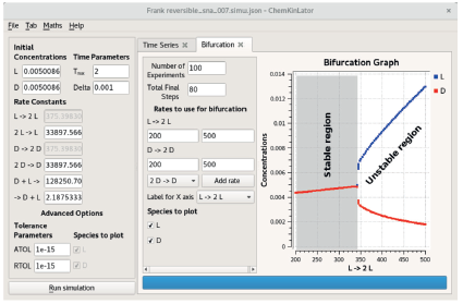
Figure 1 The bifurcation diagram of the Frank reversible model. The simulation parameters are shown on the left side of the figure, a snapshot of the Chemki„lator computer programme [16] used to make the simulations. The initial difference in the enantiomers concentration is 1 x 10-15, equivalent to an enantiomeric excess (ee) of ~ 1 x 10⁻⁹ %.
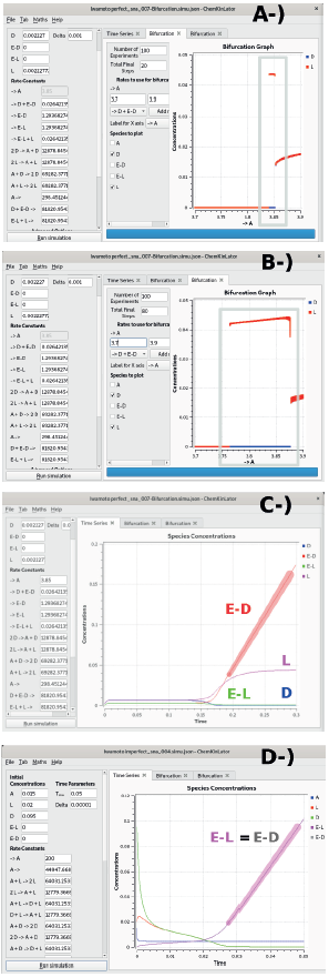
Figure 2 The Bifurcation diagrams of the Iwamoto perfect model showing A) the small unstable region when the perturbation is small (ee of order ≈ 1 x 10⁻⁵ %), and B) when the perturbation is larger, ee ≈ 2 x 10⁻² %. The time series in C) highlights the unbounded growth of the concentration of ED, and the time series in D) corresponds to the imperfect version. In C), the SMSB is evident, while in D) racemisation is evident, which means that no SMSB is produced in the imperfect model, although this second system is also unstable, due to the unlimited growth of the concentrations of EL and ED.
Frank like models
This section presents a sequence of network models derived from the Frank model. The sequence can be understood as a progression along which the original Frank model is being fixed, making it consistent with the most fundamental thermodynamic and kinetic principles.
Frank model (Frank.py, 1953)
The first ever proposed model of biological homochirality was the Frank model (2), which we present below.
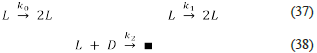
The Frank model is a network of irreversible reactions that guarantees the SMSB due to the autocatalytic reactions [37], the inhibition reaction [38], and the open condition represented by the absence of reverse reactions. The irreversibility of one reaction can be understood as a backward rate with a very low value. This can be due to low product concentration. It is also possible to understand the low backward rate as an inherent low value for the backward rate constant. Unfortunately, when someone proposes a mechanism, the reasons for removing the reverse reactions are not presented, or they are mentioned briefly. This fact can be a source of misunderstandings, given that introducing a one-way reaction violates the principle of microscopic reversibility (detailed balance) [38-41]. In that case, an improvement to the Frank model is to turn its three reactions into reversible ones, which will be carried out in the next section. For now, observe that the product of the Frank model's third irreversible reaction is irrelevant, and it does not have an explicit name; it is a generic product represented by a square, which means anything.
In conclusion, the Frank model is a network constituted of two autocatalytic (positive feedback) and one inhibition (negative feedback) reactions [42], which are irreversible. Moreover, it is an open system with an unspecified product. Frank model generates SMSB for any set satisfying the conditions k0 = k1 > 0 and k2 > 0. Thus, this is a model that always generates SMSB. These facts can be verified using Lista„alchem, second algorithm, and the file "Frank.py".
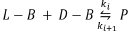
Reversible Frank model (Frank-Rev.py, this work)
The following reactions give the reversible Frank model
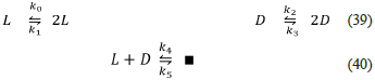
This model behaves similarly to the Frank model. However, this second model is not always unstable (as is the previous one), and only a particular set of rate constants can produce SMSB, as its bifurcation diagram shows in figure 1.
Observe that this model retains the unspecified product ∎, which, together with the reverse reaction in Eq. (40), implies a continuous input of the reagents L and D. In this way, the model satisfies the open system requirement that seems to be necessary for SMSB.
Reversible Frank model with explicit product P (Frank-Rev-P. py, this work)
The inclusion of the explicit product P in the Frank model produces:
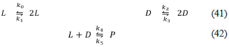
which now makes the system a closed one, and it is stable, as the second law of thermodynamics predicts. No SMSB is possible with this model. When this model is compared with the previous two, it becomes apparent that inflows of the reagents, as well as outflows of the products, are both necessary to produce instability.
A thermodynamic and kinetic consistent Frank model with two precursors (Frank-Rev-P-AB.py, this work)
Once the thermodynamic principle of detailed balance is explicit in the Frank model, some kinetics issues must be considered. First, the mass balance is not evident in reactions like those of the original Frank model Eq. (37) or the equivalent Eq. (39) and (41). Second, the first-order kinetics of those reactions are not the most common in chemistry [43]. Finally, a complete and explicit mechanism must show the origin of the enantiomeric species. The following model is a proposal to solve the aforementioned issues:
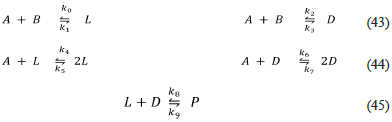
However, no SMSB is possible with this model because it is a closed system and thus a stable one. It is then reasonable to include an input of the precursor reagents A, B, and an output of the whole reaction mixture, as it is made in the classical Continuous well-Stirred Tank Reactor (CSTR) [44]. The following section presents this open system.
Open reversible Frank model with two precursors (Frank-Rev-P-AB-CSTR.py, this work)
The previous model in an open system, a standard CSTR reactor [44], can be represented as follows:
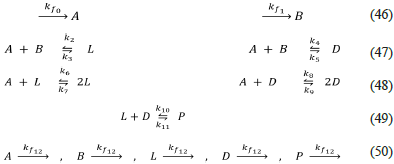
This model is thermodynamically and kinetically correct. The open system condition, a required source of instability, is included as the input Eq. (46) and output Eq. (50), which are irreversible. This model can produce homochirality, since it can be proved using SNA. However, it is important to highlight that the SNA algorithm that uses the stoichiometric matrix S Q with no extension (the process that add rows to code the duality relation between reactions), was not able to analyse this network, which has associated a large matrix of extreme currents, the matrix E Ω which has 17 rows and 25 columns. This matrix becomes, after extension, a matrix with 17 rows and only seven columns. This fact corresponds to an important characteristic of the implemented algorithm, which improves the applicability of SNA in the analysis of network models of biological homochirality. These facts can be checked using Listanalchem second algorithm, the file Frank-Rev-P-AB-CSTR.py, and changing the option "dual-pairs-in-ec" from "False" (S Q not extended) to "True" (S Ω extended).
Kondepudi-Nelson model (Kondepudi-Nelson.py, 1983)
The chronologically successive network model of homochirality is the Kondepudi-Nelson model (KN) shown below [3,4,45].
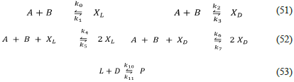
Observe that this model is essentially the same as the thermodynamic and kinetic consistent Frank model Eq. (43 - 45), except Eq. (53), which has become the irreversible inhibition Eq. (38) of the Frank model, and the trimolecular character of Eq. (52) respect to Eq. (44). Kondepudi-Nelson considers A and B as constants (i.e., they consider a pool chemical approximation [21]). This fact turns the KN model into an open system, with only two variables, Xl and X D . If reagents A and B are not constant, then two problems appear; first, the trimolecular reactions Eq. (52) are very uncommon in real systems, as well as the incapability of the model to produce SMSB; see the output of Listanalchem using the file "Kondepudi-Nelson-AS.py".
We can summarise this first set of Frank-type models comparing the most relevant aspects of them, as shown in Table 1.
Table 1 Comparison of the most relevant characteristics of the Frank-type models discussed in this work.
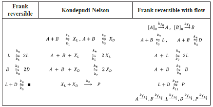
Observe that the Frank and Kondepudi-Nelson models constitute the core of the "all explicit" Frank reversible model with flow, right column on Table 1. This latter model is our proposal, and which evidences the requirements for a thermodynamic and kinetic consistent model producing SMSB. These facts are not always explicit in the literature, which is probably an important source of misunderstandings [38-41], and this is something that we want to avoid here. Of course, being so explicit has consequences: larger models and larger matrixes. However, we have partially surpassed this problem in this study, as mentioned before, using a suitable preprocessing of the stoichiometric matrixes.
Calvin model, 1969
Melvin Calvin proposed a model to explain the origin of homochirality [17,6]. His model can be presented in three different forms, as shown below.
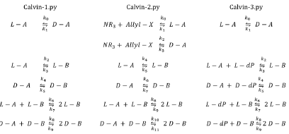
These models do not produce SMSB. Let us modify these models to make them capable of producing SMSB. First, we make them open using a CSTR, but this is not enough for the production of SMSB, as can be verified by checking the files Calvin-#-CSTR.py, where the symbol # represents one of the numbers 1, 2, or 3 that label the different versions of the Calvin model. Second, we observe that these three models have two pairs of enantiomers (L -A, D-A, and L - B, D - B), but they do not have an inhibition reaction (negative feedback) as the one in the Frank-type models. In some specific models, inhibition reactions are necessary to produce SMSB, as was proved in reference [7]. Accordingly, the three Calvin models were added with an inhibition reaction:
It was observed that SMSB is still not possible according to SNA (see files Calvin-#-CSTR-Inhibition.py, second algorithm). However, when a more specific analysis is made, using the fifth [46] and sixth [33] Listanalchem algorithms, it was found that SMSB exists in versions 2 and 3 of the model (see files Calvin-2-CSTR-Inhibition.py and Calvin-3-CSTR-Inhibition.py, fifth and sixth algorithms), but it does not appear in version 1, see file Calvin-1-CSTR-Inhibition.py. This fact means that the heuristic (the work with the minors of the current matrix Vq used in the second algorithm-SNA of Listanalchem to find the instability) is not 100 % effective, and some false negatives, like those presented before, are eventually obtained.
Nevertheless, as we have seen (and we will see with the following models), those cases are not common, making the SNA useful most of the time. Also, it is important to note, in this point, that the samples taken by the fifth and sixth Listanalchem algorithms need some minor adjustment to make the SMSB evident. Usually, it is enough to increase the perturbation of the initial enantiomeric excess or draw the bifurcation diagrams to see the range of the rate constants where the SMSB is possible. This work can be carried out using Chemkinlator (16). These facts will not be discussed in detail because it is not within the scope of this work which is dedicated only to the SNA algorithm, but those interested can use Listanalchem and Chemkinlator to explore them. The critical fact here is that the additional work needed to find SMSB in these versions of the Calvin model demonstrated that in those models, it is not easy to find SMSB.
Finally, to end with the Calvin model, we have added limited enantioselectivity (LES) reactions [47]:

instead of the inhibition reaction. The result was no SMSB is possible. However, if those four LES reactions are not forced to have the same values as the autocatalytic rate constants, as must be the case, then SMSB becomes possible in Calvin-1-CSTR-LES.py and Calvin-2-CSTR-LES.py but not in Calvin-3-CSTR-LES.py. Some authors have used this fact to obtain SMSB [18], but there is no way to justify four different rate constants for those four reactions. Thus, in conclusion, the Calvin model as initially proposed is stable.
Iwamoto model, 2003
Iwamoto proposed a reaction model including Michaelis-Menten type catalytic reactions. Iwamoto argues that his model is different from Frank and Kondepudi-Nelson's models [5]. He presented two versions of his proposal: perfect and imperfect. The latter classification is based on the stereoselectivity R1, R1a, R2, R2a, or stereospecificity R3, R3a, R4, R4a, as shown in Table 2.
Table 2 The Iwamoto model. The perfect, imperfect, and equivalent mechanisms. The equivalent mechanisms have the constant species absent according to the requirements of Listanalchem.

Iwamoto assumes constant concentrations for P, Zl, Zd, Yl, Yd and Q. Under these conditions, the mechanisms are reduced to the two columns on the right of Table 2, labeled with the expression "Equivalent to". We analysed this model using our tools (Listanalchem second algorithm - SNA).
Iwamoto perfect model (Iwamoto-Perfect.py)
The perfect version of the Iwamoto model is an open system due to the irreversible reactions R5, R6 and also to the reversibility of the reactions that have either constant (not explicit) reagents or constant products (reactions R0, R3, R4). These reactions, together with the autocatalytic reactions (positive feedback) R1, R2, and the negative feedback given by reactions R3, R4 (the consumption of the isomeric-autocatalytic species), make this model capable of producing SMSB. Notwithstanding, the region where the model is unstable is small, as Figure 2 shows.
In Figure 2 A, the initial difference between the concentrations of the two enantiomers, the enantiomeric excess (ee), is of order 1 x 10⁵ %. If the initial difference between those concentrations increases to ee ≈ 2 x 10 2 %, we can observe a larger instability region in the bifurcation diagrams, as shown in Figure 2 B. On the other hand, we have to observe that this model shows an unbounded growth of the concentration of the Ed species, Figure 2 C.
Iwamoto imperfect model (Iwamoto-Imperfect.py)
If we add to the perfect model the imperfect stereoselectivity reactions R1a, R2a, and the imperfect stereospecificity reactions R3a, R4a, we get the imperfect model. When the tuples R1, Ria, R2, R2a, and R3, R3a, R4, R4a have the same rate constants, then the Listanalchem programme, SNA algorithm, finds an unstable region. However, the values sampled for the rate constants cannot produce SMSB, and the bifurcation diagrams show no SMSB in the neighbourhood of those values. The detected instability is due to the unlimited growth of the concentrations of El and Ed, Figure 2 D. Nevertheless, it is possible to obtain a model capable of SMSB by using the same trick used in the analysis of the three Calvin models: we allow different values for the rate constants of Ria, R2a with respect to values of the rate constants of Ri, R2, and we do the same for the pairs R3a, R4a, and R3, R4. However, it is unclear why those rate constants could be different, given that the reagents are the same.
APED model (APED.py, 2004)
The model proposed in reference [18], and called APED model, is shown below:

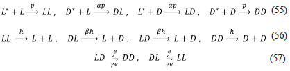
According to the model's authors, the rate constants of reactions (55) must be different p ≠ αp, as well the rate constants of reactions (56) h ≠ βh, and reactions (57) e ≠ γe. Under these circumstances the APED model produces SMSB (in Listanalchem, second algorithm - SNA, "instability-heuristic": "characteristic-polynomial" must be used instead of "instability-heuristic": "mineurs"). However, it is hard to justify those differences, as mentioned before in the analysis of Calvin and Iwamoto's models, but as it was also mentioned, those differences are adequate to obtain SMSB as the APED model confirms. Moreover, the authors of the APED model seem to be conscious of this fact since they give those rate constants the same name times a factor.
The differences between those rate constants are so efficient in producing SMSB that even when the reactions (55), (56) turn reversible, the model still presents SMSB. However, it is not found using SNA alone, the algorithm presented here. That requires additional work that will not be discussed because it is not within the scope of this study, but it can be revised using the Listanalchem sixth algorithm [33] and Chemkinlator (see file APED-Reversible.py).
In conclusion, the APED model does not generate SMSB when the rate constants of the equivalent (dual) reactions (55) dimerisation and (56) depolymerisation are equal (between them), a = p = 1.
Replicator model of Hochberg and Ribo (Replicator-HR.py, 2019)
Hochberg and Ribo [48] proposed the following network
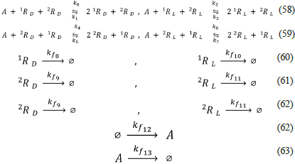
A relevant characteristic of this model is its ability to produce SMSB when all the equivalent (dual) reactions have the same rate constants: k 0 = k 2 = k 4 = k 6 , and k 1 = k 3 = k 5 = k 7 . This important feature is not observed in previous models. Nevertheless, the trimolecular character of reactions (58) and (59) is problematic from the point of view of kinetics. On the other hand, we would like to observe that this model fulfils the previously mentioned requirements for producing SMSB: positive feedback (autocatalysis), negative feedback (the autocatalytic species in reactions (58) are not in reactions (59), and vice versa), and the open character represented by the irreversible pseudo-reactions (60) to (63).
Chaotic replicator model of Hochberg, Sánchez and Morán (Chaotic-Replicator-Hochberg-et-al-2020.py, 2020)
The chaotic replicator [49] includes four enantiomeric pairs (i = 1, 2, 3, 4), autocatalysis, the same kind of negative feedback present in the previous model, irreversible reactions, and a CSTR (see below).
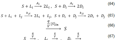
This model is particular because, additional to SMSB, it exhibits chaotic behaviour. This chaotic behaviour occurs when one sets the values of the rate constants to pertain to a very particular range, which usually includes a small interval (0 to ≈ 0.06) for a couple of the rate constants (65); e.g. S + L
2
+
 However, the probability of finding this small region using our heuristic based on random sampling is low, which is not a drawback because this algorithm was not designed to detect chaos but SMSB. This small region of the rate space was found using the bifurcation diagram option of the Chemkinlator software (16) and the rate constants proposed in reference [49].
Kondepudy-Mundy radiation activated model (Kondepudy-Mundy-2020.py, 2020)
Kondepudy and Mundy have presented a model, which can be considered an update of the old Kondepudi-Nelson model [50]. This new model solves the previously mentioned issues of the old model. Kondepudi and Mundy make the system reversible and open by way of the introduction of radiation, which is also supposed to trigger the chemical reactions (as presented below on the left side).
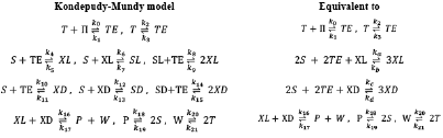
The proponents of this model also introduced some restrictions to obtain SMSB, namely: k
4
=k
6
x k
8
, k
5
=k
7
x k
9
, =x k
14
, and k
11
= x k
15
. Those equations make the model become equivalent to the network presented on the right side of the previous mechanism. We had to make explicit this equivalence because Listanalchem cannot handle those restrictions. Nevertheless, the remarkable fact is that our algorithm was able to detect SMSB in the updated KN model, which is a likely result, taking into account the external input of the radiation n, as well as the presence of the autocatalytic and inhibition reactions of the well studied Kondepudy-Nelson model (on which this new model is based). Finally, we want to mention that there is an error in the description of the first reaction reported in reference (50), Table 1, because it says
 and it must be
 It is important to mention that we detected this error thanks to our computer programme Listanalchem second algorithm-SNA, which allowed us to test the stability of these two options efficiently.
Blackmond chemical review (Blackmond-Rev-2020.py, 2020)
Blackmond discusses, in her 2020 review, the modelling of the Soai reaction (40). The following mechanism readily resumes her proposal.
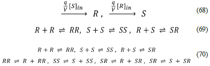
This network exhibits some of the features that allow the emergence of homochirality: external input of the precursors (irreversible pseudo-reactions) although not an explicit output, autocatalysis (RR ⇌ R + RR, SS ⇌ S + SS), and negative feedback R+S ⇌ SR, which produces the heterochiral inactive catalytic species SR. The specific scheme presented above was elaborated with the help of our SNA algorithm because the original scheme 8, presented by Blackmond in her review, was shown (using our algorithm) incapable of producing SMSB. We want to remark that this is one of the capabilities of our algorithm: it can lead us in the design (and improvement) of network models of biological homochirality.
The Soai reaction mechanism proposed by Trapp and co-workers (Soai-Trapp-et-al.py, 2020)
Trapp and co-workers presented a reaction mechanism that is supposed to model the Soai reaction [19]. This mechanism was constructed from a large set of experimental data. This model includes 26 species and 34 reactions (counting forward and reverse), too large to be shown here, but available in the reference as well as in the file "Soai-Trapp-et-al.py" of Listanalchem folder "models". We have to say that our SNA algorithm classified the network as incapable of SMSB. However, if one uses Chemkinlator on the set of parameter values provided in [19], it will observe SMSB. This fact can be seen as a fault of our algorithm, which should rely on the approximate nature of the algorithms used to solve the nonlinear inequalities in the analysis. However, we would like to stress the capability of our algorithm in handling such a huge mechanism. Also, as was shown when the Calvin models were discussed, additional analysis can be carried out using the Listanalchem fifth algorithm. That one allows founding SMSB in this enormous mechanism. However, as before with the Calvin model, no more discussion will be presented here because the scope of this work is only the SNA algorithm.
Conclusions
The mathematical tools provided by Clarke's Stoichiometric network analysis were implemented as a computer programme. This implementation allows us to focus the stability analysis on the matrixes of extreme currents, whose entries are linear polynomials and not the nonlinear polynomials that occur as entries of the Jacobian matrixes. This fact allows us to efficiently search the instability sources of the coupled systems of differential equations that govern the chemical mechanism proposed to explain the chemistry behind the emergence of homochirality.
The algorithm and the computer programme presented here were used to analyse ten different models of biological homochirality that appear in the related literature and 18 variations of those models for a total of 28 models. This was possible thanks to the efficiency of our algorithm.
This work allows us to detect some of the sources of SMSB, namely: autocatalysis (positive feedback), negative feedback (usually presented as inhibition reactions that involve two enantiomers), and openness (similar to CSTR, but also representable by irreversible reactions which are usually not well supported). Furthermore, we observed that these sources of instability are generally present in the models proposed in the literature, and we studied the consequences of adjusting some of them to the basic principles of thermodynamics and kinetics.

