Inglés (pdf)
 Articulo en XML
 Referencias del artículo
 Enviar articulo por email
 Citado por SciELO
  Citado por Google
  Similares en
SciELO
Similares en
SciELO  Similares en Google
 Permalink
1. Introduction
The study of the dynamics of a fragmented population is fundamental in theoretical ecology, with potentially very important applied aspects: what is the effect of migration on the general population dynamics? What are the consequences of fragmentation on the persistence or extinction of the population? When is a single large refuge better or worse than several small ones (this is known as the SLOSS debate; see Hanski [19])?
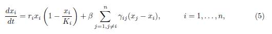
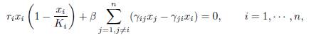
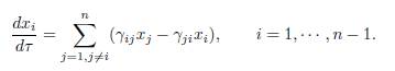
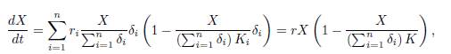
The theoretical paradigm that has been used to treat these questions is that of a single population fragmented into patches coupled by migration, and the sub-population in each patch follows a local logistic law. This system is modeled by a non-linear system of differential equations of the following form:
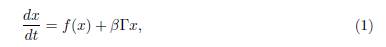
where x = (x1, . . . , xn)T , n is the number of patches in the system, xi represents the population density in the i-th patch, f(x) = (f1(x1), . . . , fn(xn))T , and

The parameters ri and Ki are respectively the intrinsic growth rate and the carrying capacity of patch i.
The term βΓx on the right hand side of the system (1) describes the effect of the mi-gration between the patches, where β is the migration rate and Γ = (γij) is the matrix representing the migrations between the patches. For i # j, γij > 0 denotes the incoming flux from patch j to patch i. If γij = 0, there is no migration. The diagonal entries of Γ satisfy the following equation
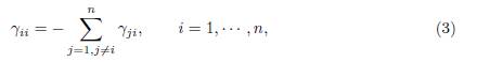
which means that what comes out of a patch is distributed between the other n − 1 patches.
In the absence of migration, (β = 0), the system (1) admits (K1, . . . , Kn) as a non-trivial equilibrium point. This equilibrium is globally asymptotically stable (GAS) and the total population at equilibrium is equal to the sum of the carrying capacities. The problem is whether or not the equilibrium continues to be positive and GAS, for any β > 0, and whether or not the total population at equilibrium can be greater than the sum of the carrying capacities. The case n = 2 and Γ symmetric
where γ12 = γ21 is normalized to 1 has been considered by Freedman and Waltman [14] and Holt [18]. They analyzed the model in the case of perfect mixing (β → +∞) and showed that the total equilibrium population can be greater than the sum of the carrying capacities K1 + K2, so that patchiness has a beneficial effect on the total equilibrium population. More recently, Arditi et al. [1] analyzed the behaviour of the system for all values of β. They showed that only three situations occur: either for any β > 0, patchiness has a beneficial effect, or this effect is always detrimental, or the effect is beneficial for lower values of the migration coefficient β and detrimental for higher values. Arditi et al. [2] extended these results to the case of two patches coupled by asymmetric migration, corresponding to the matrix
See also Poggiale et al. [25] who considered two patches coupled by asymmetric migration, in the particular case of perfect mixing. DeAngelis et al. [8, 11] considered the case of n > 2 patches in a circle, with symmetric migration between any patch and its two neighbours :
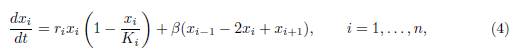
where we denote x0 = xn and xn+1 = x1, so that the same relationships hold between xi, xi−1 and xi+1 for all values of i. This model corresponds to the matrix Γ whose non-zero off-diagonal elements are given by

The system (4) is a one-dimensional discrete-patch version of the standard reaction-diffusion model. In [8, 11] the perfect mixing case is described.
In [12] we considered the general symmetric migration. We studied the system:
where βγij is the rate of migration between patches i and j. This system can be written in the form of System (1) with Γ = (γij), the symmetric matrix whose diagonal entries are defined by (3). We studied the total population at equilibrium, as a function of the migration rate β. We gave conditions on the system parameters that ensure that migration is beneficial or detrimental, and extended several results of [1, 8, 11].
The aim of this work is to consider the case of n patches connected by asymmetric migration. Thus, we extend [2] by considering the case n ≥ 2, and we extend [12] by considering the case where Γ is non-symmetric.
An important extension of (1) is the so called source-sink model, where the patches are of two types: the source patches, 1 ≤ i ≤ m, with logistic dynamics, and the sink patches, m + 1 ≤ i ≤ n, with exponential decay
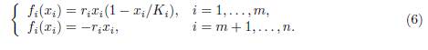
The main problem is the number of source patches required for population persistence. For a recent study and bibliographical references the reader can consult Arino et al. [3] and Wu et al. [30].
There is another important extension of (1,2), where the dynamics on patch i is of the form

with γi > 0. This model is the limit system (when t → +∞) of a susceptible-infected-susceptible (SIS) model in n patches connected by human migration. For details and further reading, see Section 5. Note that, when ri < γi for some patches, system (1,7) is a source-sink model. Countrary to (6), the mortality in sink patch is density-dependent. For more details and bibliographical references the reader is referred to [15].
Another example of source-sink model is the system considered by Nagahara et al. [24], called the “island chain” model, which is of the form:

where we denote x0 = x1 and xn+1 = xn. This model is of the form (1), Γ being the matrix which verifies (3), and whose non-zero off-diagonal elements are given by
In the model (8) the ratios αi = ri/Ki in (2) are equal and are normalized to 1. The constant mi represents both the intrinsic growth rate of the species in patch i and the carrying capacity of the patch. If mi > 0, then patch i is favorable to the species. It is a source. The case mi = 0 is permitted and corresponds to a sink. The main purpose is to find the resource allocation (m1, ..., mn) that maximizes the total population at equilibrium, under the constraint that Σi mi = m > 0 is fixed. For more details and information on the maximization of the total population with logistic growth in a patchy environment, the reader is referred to [24] and the references therein.
For general information of the effects of patchiness and migration in both continuous and discrete cases, and the results beyond the logistic model, the reader is referred to the work of Levin [20, 21], DeAngelis et al. [8, 9, 10, 11], Freedman et al. [13], Zaker et al. [33].
It is worth noting that System (1) appears in metapopulation dynamics, involving explicit movements of the individuals between distinct locations. For the graph theoretic and dynamical system context in which metapopulation models are formulated, the reader is referred to Arino [4, Section 2].
The paper is organized as follows. In Section 2, the mathematical model of n patches, and some preliminaries results, are introduced. In Section 3, the behavior of the model is studied when the migration rate tends to infinity. In Section 4, we compare the total equilibrium population with the sum of the carrying capacities in some particular cases. In Section 5, the SIS patch model is considered, and the links with the logistic patch model are investigated. In Section 6 the three-patch model is considered, and by numerical simulations we show the existence of a new behavior for the dynamics of the total equilibrium population as a function of the migration rate. In Appendix A, we recall some results for the two-patch model with asymmetrical migration. In Appendix B, we prove some useful auxiliary results.
2. The mathematical model and preliminaries results
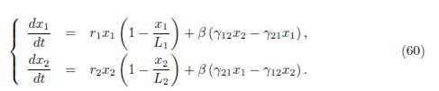
We consider the model of multi-patch logistic growth, coupled by asymmetric migration terms
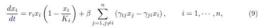
where γij ≥ 0 denotes the incoming flux from patch j to patch i, for i # j. The system (9) can be written in the form (1), where f is given by:

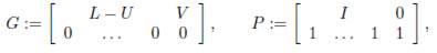
and Γ := (γij)n×n is the matrix whose diagonal entries are given by (3). The matrix
which is the same as Γ, except that the diagonal elements are 0, is called the connectivity matrix. It is the adjacency matrix of the weighted directed graph G, which has exactly n vertices (the patches), and has an arrow from patch j to patch i, with weight γij, precisely when γij > 0.
As to the non-negativity of the solution, we have the following proposition:
Proposition 2.1. The domain ℝ n + = {(x1, . . . , xn) ∈ ℝ n/xi ≥ 0, i = 1, . . . , n} is positively invariant for the system (9).
Proof. The proof is the same as in the symmetrical case [12, Proposition 2.1].
When the connectivity matrix Γ0 is irreducible, System (9) admits a unique positive equilibrium (x∗ 1(β), . . . , x∗ n(β)), which is GAS, see [4, Theorem 2.2], [3, Theorem 1] or [12, Theorem 6.1]. In all of this work, we denote by E∗(β) the positive equilibrium and by XT ∗ (β) the total population at equilibrium:
Remark 2.2. The matrix Γ0 being irreducible means that the weighted directed graph G is strongly connected, which means that every patch is reachable from every other patch, either directly or through other patches. The matrix Γ is assumed to be irreducible throughout the rest of the paper.
3. Perfect mixing
In this section our aim is to study the behavior of E∗(β) and XT ∗ (β), defined by (11), for large migration rate, i.e when β → ∞.
3.1. The fast dispersal limit
The following lemma was proved in [3, Lemma 2]; we include a proof for the ease of the reader.
Lemma 3.1. Let Γ be the migration matrix. Then, 0 is a simple eigenvalue of Γ and all non-zero eigenvalues of Γ have negative real part. Moreover, the kernel of the matrix Γ is generated by a positive vector. If the matrix Γ is symmetric, then ker Γ is generated by u = (1, ..., 1)T .
Proof. Let s = maxi=1,...,n(−γii) and let B be the matrix defined by
First, we note that since the matrix Γ verifies the property (3), then Γ is a singular matrix and the vector u = (1, ..., 1)T is an eigenvector of ΓT associated to the eigenvalue 0. Thus u is an eigenvector of BT , with eigenvalue s.
The matrix BT is non-negative and irreducible, so by the Perron-Frobenius Theorem the spectral radius
is a simple eigenvalue of the matrix BT and it is the only eigenvalue of BT which admits a positive eigenvector, so s = ρ(BT ) = ρ(B). Therefore, Γ = B −ρ(B)I and dim(ker Γ) = dim(ker ΓT ) = 1.
All other eigenvalues of B have modulus < ρ(B), so their real parts are < ρ(B). Since each eigenvalue of Γ is λ − ρ(B), for some eigenvalue λ of B, all eigenvalues of Γ have negative real part.
Furthermore, according to the Perron-Frobenius theorem, there exists a positive vector δ such that Bδ = ρ(B)δ, that is, Γδ = (B − ρ(B)I)δ = 0. In particular, if the matrix Γ is symmetric then we may take δ = u, that is, δi = 1, for all i.
In all of this paper, we denote by δ = (δ1, . . . , δn)T a positive vector which generates the vector space ker Γ.
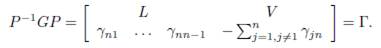
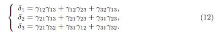
Remark 3.2. The existence, uniqueness (mod. multiplicative factor), and positivity of δ were also proved in Lemma 1 of Cosner et al. [5]. On the other hand, it is shown in Guo et al. [17, Lemma 2.1] and Gao and Dong [16, Lemma 3.1] that the vector (Γ∗ 11, . . . , Γ∗ nn)T is a right eigenvector of Γ associated with the zero eigenvalue. Here, Γ∗ ii is the cofactor of the i-th diagonal entry of Γ. Therefore, we have explicit formulae for the components of the vector δ, as functions of the coefficients of Γ, at our disposal. For two patches we have δ = (γ12, γ21)T , and for three patches we have δ = (δ1, δ2, δ3)T , where
The following result asserts that when β → ∞, the equilibrium E∗(β) converges to an element of ker Γ.
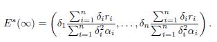
Theorem 3.3. For the system (9), we have
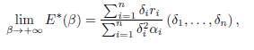
where αi = ri/Ki.
Proof. Denote
Dividing Equation 1 at the equilibrium E∗(β) by β, for β > 0, yields
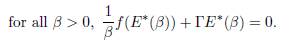
Thus any limit point, when β → ∞, of the set {E∗(β) : β > 0} lies in the kernel of Γ. Now, taking the sum of all equations in
we see that E∗(β) lies in the ellipsoid
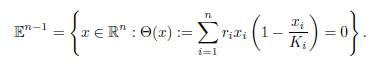
The ellipsoid 𝔼n−1 is compact, so the equilibrium E ∗(β) has at least one limit point in 𝔼n−1, when β goes to infinity. Since the kernel of Γ has dimension 1, and 𝔼n−1 is the boundary of a convex set, 𝔼n−1 ∩ ker Γ consists of at most two points. Since the origin and E∗(∞) both lie in 𝔼n−1 ∩ ker Γ, we get that

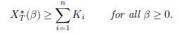
Therefore, to prove the convergence of E∗(β) to E∗(∞), it suffices to prove that the origin cannot be a limit point of E∗(β). We claim that for any β, there exists i such that x∗ i(β) ≥ Ki, which entails that E ∗(β) is bounded away from the origin. The coordinates of the vector ΓE∗(β) sum to zero, hence at least one of them, say, the i-th, is non-negative. Then
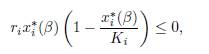
and since x∗ i (β) cannot be negative or 0, we have x∗ i (β) ≥ Ki.
As a corollary of the previous theorem, we obtain the following result, which describes the total equilibrium population for perfect mixing:
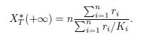
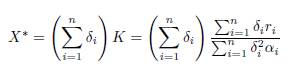
Proposition 3.4. We have
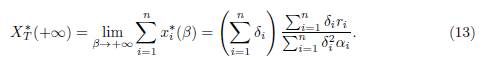
Denote K = (K1, . . . , Kn)T . If K = λδ with λ > 0, that is to say K ∈ ker Γ, then XT ∗(+∞) = λ Σn i=1 δ i = Σ n i=1 K i .
Proof. For the proof of (13), it suffices to sum the n components of the point E∗(∞). For the case K ∈ ker Γ, it suffices to replace Ki by λδi in (13).
Actually, when K ∈ ker Γ, we have X∗ T (β) =Σi Ki for all β > 0, see roposition 4.5.
In the case n = 2, one has δ1 = γ12 and δ2 = γ21, as shown in Remark 3.2. Therefore, (13) becomes
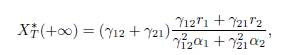
which is the formula given by Arditi et al. [2, Equation 7] and by Poggiale et al. [25, page 362].
If the matrix Γ is symmetric, one has δi = 1, for all i, as shown in Lemma 3.1. Therefore, (13) specializes to the formula given in [12, Equation (24)]:
3.2. Two time scale dynamics
In [12] we also obtained the formula (13), in the symmetrical n-patch case (i.e the matrix Γ is symmetric), by using singular perturbation theory, see [12, Theorem 4.6].
We showed that, if (x1(t, β), . . . , xn(t, β)) is the solution of (5), with initial condition (x0 1, . . . , x0 n), then, when β → ∞, the total population xi(t, β) is approximated by X(t), the solution of the logistic equation

with initial condition X0 = Σx0
i. Therefore, the total population behaves like the solution of the logistic equation given by (14). In addition, one obtains the following property: with the exception of a small initial interval, the population densities xi(t, β) are approximated by X(t)/n, see [12, Formula (37)]. Therefore, this approximation shows that, when t and β tend to ∞, the population density xi(t, β) tends toward
 and in addition, xi(t, β) quickly jumps from its initial condition x0
i to the average X0/n and then is very close to X(t)/n. Our aim is to generalize this result for the asymmetrical n-patch model (9) (i.e the matrix Γ is non-symmetric). To avoid any confusion with X(t), which is the total population, we denote Y (t) the solution of the logistic equation (15), and we prove that X(t) is asymptotically equivalent, when β goes to infinity, to Y (t). We have the following result
and in addition, xi(t, β) quickly jumps from its initial condition x0
i to the average X0/n and then is very close to X(t)/n. Our aim is to generalize this result for the asymmetrical n-patch model (9) (i.e the matrix Γ is non-symmetric). To avoid any confusion with X(t), which is the total population, we denote Y (t) the solution of the logistic equation (15), and we prove that X(t) is asymptotically equivalent, when β goes to infinity, to Y (t). We have the following result
Theorem 3.5. Let (x1(t, β), . . . , xn(t, β)) be the solution of the system (9) with initial condition (x0 1, · · · , x0 n) satisfying x0 i ≥ 0 for i = 1 · · · n. Let Y (t) be the solution of the logistic equation
Where
with initial condition X0 Σn i=1 x0 i. Then, when β → ∞, we have
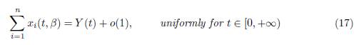
and, for any t0 > 0, we have

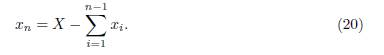
Proof. Let X(t, β) = Σn i=1 xi(t, β). We rewrite the system (9) using the variables (X, x1, ・ ・ ・ , xn−1), and get:
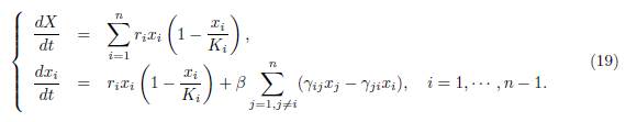
This system is actually a system in the variables (X, x1, · · · , xn−1), since, whenever xn appears in the right hand side of (19), it should be replaced by
When β → ∞, (19) is a slow-fast system, with one slow variable, X, and n − 1 fast variables, xi for i = 1 · · · n − 1. As suggested by Tikhonov’s Theorem [22, 28, 31], we consider the dynamics of the fast variables in the time scale τ = βt. We get
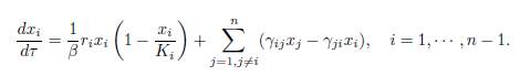
where xn is given by (20). In the limit β → ∞, we find the fast dynamics
This is an (n − 1)-dimensional linear differential system in the variable Z :=(x1, ・ ・ ・ , xn−1), which can be rewritten in matricial form:

where L := (γij)n−1×n−1 is the sub matrix of the matrix Γ, obtained by dropping the last row and the last column of Γ, V is the vector defined by V := (γin)n−1×1 and U= (V;...;V).
By Lemma B.1, the matrix ℒ is stable, that is, all of its eigenvalues have negative real part. Therefore, it is invertible and the equilibrium of the system (21) is GAS. This equilibrium is given by
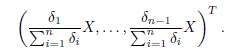
Indeed, we denote by L(i), U(i) and V (i) the i-th row of the matrix L, U and the vector V respectively. We have:
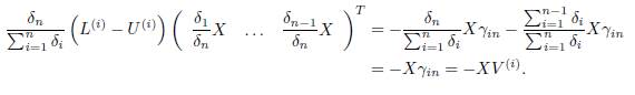
Thus, the slow manifold of System (19) is given by
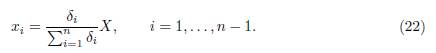
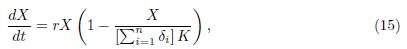
As this manifold is GAS, Tikhonov’s Theorem ensures that after a fast transition toward the slow manifold, the solutions of (19) are approximated by the solutions of the reduced model, which is obtained by replacing (22) into the dynamics of the slow variable, that is:
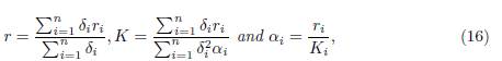
where r and K are defined in (16). Therefore, the reduced model is (15). Since (15) admits
as a positive equilibrium point, which is GAS in the positive axis, the approximation given by Tikhonov’s Theorem holds for all t ≥ 0 for the slow variable and for all t ≥ t0 > 0 for the fast variables, where t0 is as small as we want. Therefore, letting Y (t) be the solution of the reduced model (15) with initial condition Y (0) = X(0, β) = Σn i=1 x0 i , then, when β → ∞, we have the approximations (17) and (18).
In the case of perfect mixing, the approximation (17) shows that the total population behaves like the solution of the single logistic equation (16) and then, when t and β tend to ∞, the total population Σ xi (t, β) tends toward (
 as stated in Proposition 3.4. The approximation (18) shows that, with the exception of a thin initial boundary layer, where the population density xi(t, β) quickly jumps from its initial condition xi
0 to δiX0/ Σn
i=1 δi, each patch of the n-patch model behaves like the logistic equation
as stated in Proposition 3.4. The approximation (18) shows that, with the exception of a thin initial boundary layer, where the population density xi(t, β) quickly jumps from its initial condition xi
0 to δiX0/ Σn
i=1 δi, each patch of the n-patch model behaves like the logistic equation

Hence, when t and β tend to ∞, the population density xi(t, β) tends toward
 δi as stated in Theorem 3.3.
Remark 3.6. The single logistic equation (23) gives an approximation of the population density in each patch in the case of perfect mixing. The intrinsic growth rate r in (23) is the arithmetic mean of the r1, . . . , rn, weighted by δ1, . . . , δn, and the carrying capacity K is the harmonic mean of Ki/δi, weighted by δiri, i = 1, . . . , n. We point out the similarity between our expression for the carrying capacity in the limit β → ∞, and the expression obtained in spatial homogenization, see e.g [32, Formula 81] and also [33, Formula 28].
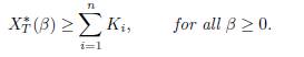
3.3. Comparison of XT ∗ (+∞) with Σi Ki.
According to Formula (13), it is clear that the total equilibrium population at β = 0 and at β = +∞ are different in general.
In the remainder of this section, we give some conditions, in the space of parameters ri, Ki, αi and δi, for limit of the total equilibrium population when β → ∞ to be greater or smaller than the sum of the carrying capacities. We show that all three cases are possible, i.e XT ∗ (+∞) can be greater than, smaller than, or equal to XT ∗ (0). First, we start by giving some particular values of the parameters for which equality holds.
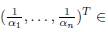
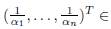
Proposition 3.7. Consider the system (9). If the vector
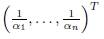 lies in ker Γ, hen XT
∗ (+∞) = i Ki.
lies in ker Γ, hen XT
∗ (+∞) = i Ki.
Proof. It is a direct consequence of the Equation (13).
Note that, if the matrix Γ is symmetric, then by Lemma 3.1, Proposition 3.7 says that if all αi are equal, then XT ∗ (∞) = Σi Ki, which is [12, Proposition 4.4].
In the next proposition, we give two cases which ensure that XT ∗ (0) can be greater or smaller than XT ∗ (+∞). This result can be stated as the following proposition:
Proposition 3.8. Consider the system (9).
In both items, if at least one of the inequalities in
 is strict, then the inequality is strict in the conclusion.
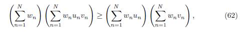
Proof. Apply Lemma B.2 with the following choice:
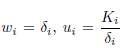 and vi = δiαi, δi, for all i = 1, . . . , n.
If the matrix Γ is symmetric, one has δi = 1, for all i, as shown in Lemma 3.1. Therefore Proposition 3.8 becomes
Corollary 3.9. Consider the system (9). Assume that Γ is symmetric.
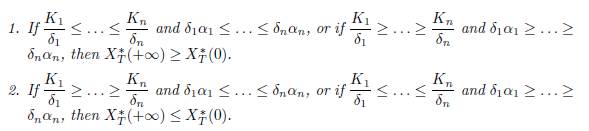
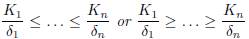
If K1 ≤ . . . ≤ Kn and α1 ≤ . . . ≤ αn, or if K1 ≥ . . . ≥ Kn and α1 ≥ . . . ≥ αn, then XT ∗ (+∞) ≥ XT ∗ (0).
If K1 ≥ . . . ≥ Kn and α1 ≤ . . . ≤ αn, or if K1 ≤ . . . ≤ Kn and α1 ≥ . . . ≥ αn, then XT ∗ (+∞) ≤ XT ∗ (0).
This result implies Items 1 and 2 of [10, Theorem B.1], which were obtained for the model (4) in the particular case ri = Ki.
4. Influence of asymmetric dispersal on total population size
In this section, we will compare, in some particular cases of the System (9), the total equilibrium population XT ∗ (β) = x∗ 1(β) + . . . + x∗ n(β), with the sum of carrying capacities denoted by XT ∗ (0) = K1 + . . . + Kn, when the rate of migration β varies from zero to infinity. We show that the total equilibrium population, XT ∗ (β), is generally different from the sum of the carrying capacities XT ∗ (0). Depending on the local parameters of the patches and the kernel of the matrix Γ, XT ∗ (β) can either be greater than, smaller than, or equal to the sum of the carrying capacities.
4.1. Asymmetric dispersal may be unfavorable to the total equilibrium population
When Γ is symmetric, we have already proved that if all the growth rates are equal then dispersal is always unfavorable to the total equilibrium population, see [12, Proposition 3.1]. We also noticed that the result still holds in the general case when Γ is not necessarily symmetric, see [12, Proposition 6.2]. Hence we have the following
Proposition 4.1. If r1 = . . . = rn then
For a two-patch logistic model, this result has been proved by Arditi et al. [1, Proposition 2, item 3] for symmetric dispersal and for asymmetric dispersal [2, Proposition 1, item 3].
4.2. Asymmetric dispersal may be favorable to the total equilibrium population
In this section, we give a situation where the dispersal is favorable to the total equilibrium population. Mathematically speaking:
Proposition 4.2. Assume that for all j < i, αiγij = αjγji. Then
Moreover, if there exist i0 and j0 # i0 such that ri0 # rj0 , then XT ∗ (β) > Σn i=1 all β > 0.
Proof. The equilibrium point E∗(β) satisfies the system
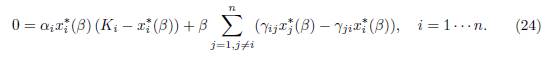
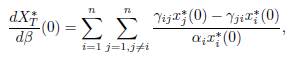
Dividing (24) by αix∗ i, one obtains
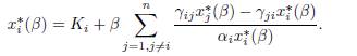
Taking the sum of these expressions shows that the total equilibrium population XT ∗ satisfies the following relation:
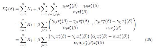
The conditions αiγij # αjγji can be written κij: = αi/γji # αj/γij for all j < i, such that γij # 0 and γji # 0. Therefore, there exists κij > 0 such that

Replacing αi and αj in (25), one obtains
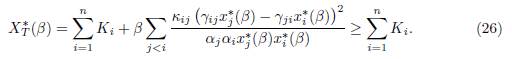
Equality holds if and only if β = 0 or γijx∗ j(β) − γjix∗ i(β) = 0, for all i and j. Let us prove that if at least two patches have different growth rates, then equality cannot hold for β > 0. Suppose that there exists β∗ > 0 such that the positive equilibrium satisfies

Replacing the Equation (27) in the system (24), we get that x∗ i(β∗) = Ki, for all i. Therefore, from (27), it is seen that, for all i and j, Kjγij = Kiγji. From these equations and the conditions αiγij = αjγji, we get ri = rj, for all i and j. This is a contradiction with the hypothesis that there exist two patches with different growth rates. Hence the equality in (26) holds if and only if β = 0.
When the matrix Γ is irreducible and symmetric, the hypothesis of Proposition 4.2 implies that αi = αj for all i and j. Indeed if two patches i and j are connected (i.e γij = γji ̸= 0), then we have αi = αj. As the matrix Γ is irreducible, for two arbitrary patches, there exists a finite sequence (i, . . . , j) which begins in i and ends in j, such that γab ̸= 0 for all successive patches a and b in (i, . . . , j). Hence αa = αb for all a and b in (i, . . . , j). Hence, αi = αj. So, when the matrix Γ is symmetric, Proposition 4.2 says that if all αi are equal, dispersal enhances population growth, which is [12, Proposition 3.3].
Note that, when n = 2, Proposition 4.2 asserts that if α2/α1 = γ12/γ21, then XT ∗ (β) > K1 + K2, which is a result of Arditi et al. [2, Proposition 2, item b]. See also Proposition A.1, and note that the condition α2/α1 = γ12/γ21 implies that (γ12, γ21) ∈ J0.
For three patches or more, if the matrix Γ does not verify the condition (∀i, j, γij = 0 ⇐⇒ γji = 0), then the hypothesis of Proposition 4.2, that for all j < i, αiγij = αjγji cannot be satisfied. Note that the hypothesis αiγij = αjγji implies that, for all i = 1, . . . , n, one has
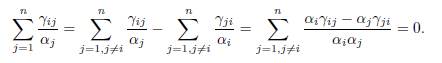
Therefore we can make the following remark:
Remark 4.3. The hypothesis of Proposition .2 implies that
 ker Γ.
We make the following conjecture:
Conjecture. If
 ker Γ then
This conjecture is true for the particular case of Proposition 4.2. It is also true for two-patch models and for n-patch models with symmetric dispersal. It agrees with Proposition 3.7.
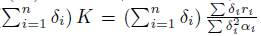
Proposition 4.4. The derivative of the total equilibrium population XT ∗ (β) at β = 0 is given by:
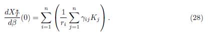
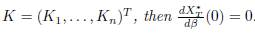
In particular, if K ∈ ker Γ, where
Proof. By differentiating the Equation (25) at β = 0, we get:
which gives (28), since x∗ i(0) = Ki for all i = 1, . . . , n.
If K ∈ ker Γ, then Σn
j=1 γijKj = 0 for all i, so that
 .
.
Actually, when K ∈ ker Γ, we prove that X∗
T (β) is constant, so that
 for allΒ ≥ 0, not only for β = 0, see Proposition 4.5.
4.3. Independence of the total equilibrium population with respect to asymmetric dispersal
In the next proposition we give sufficient and necessary conditions for the total equilib-rium population not to depend on the migration rate.
Proposition 4.5. The equilibrium E∗(β) does not depend on β if and only if (K1, . . . , Kn)T ∈ ker Γ. In this case, we have E∗(β) = (K1, . . . , Kn) for all β > 0.
Proof. The equilibrium E∗(β) is the unique positive solution of the equation
where f is given by (10). Suppose that the equilibrium E∗(β) does not depend on β, then we replace in Equation (29):
The derivative of (30) with respect to β gives

Replacing the Equation (31) in the Equation (30), we get f(E∗(β)) = 0, so E∗(β) = (K1, . . . , Kn). From the Equation (31), we conclude that (K1, . . . , Kn)T ∈ ker Γ.
Now, suppose that (K1, . . . , Kn)T ∈ ker Γ, then (K1, . . . , Kn) satisfies the Equation (29), for all β ≥ 0. So, E∗(β) = (K1, . . . , Kn), for all β ≥ 0, which proves that the total equilibrium population is independent of the migration rate β.
If the matrix Γ is symmetric, the previous proposition asserts that the Ki, for i = 1, . . . , n, are equal if and only if E∗ = (K, . . . , K), where K is the common value of the Ki. This is [12, Proposition 3.2]. For n = 2 , Proposition 4.5 asserts that if K1/K2 = γ12/γ21 then XT ∗ (β) = K1 + K2 for all β, which is [2, Proposition 2, item c ]. See also the last item of Proposition A.1.
4.4. Two blocks of identical patches
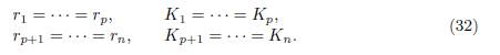
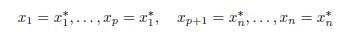
We consider the model (9) and we assume that there are two blocks, denoted I and J, of identical patches, such that I ∪ J = {1, · · · , n}. Let p be the number of patches in I and q = n − p be the number of patches in J. Without loss of generality we can take I= {1, · · · , p} and J = {p + 1, · · · , n}. The patches being identical means that they have the same specific growth rate ri and carrying capacity Ki. Therefore we have
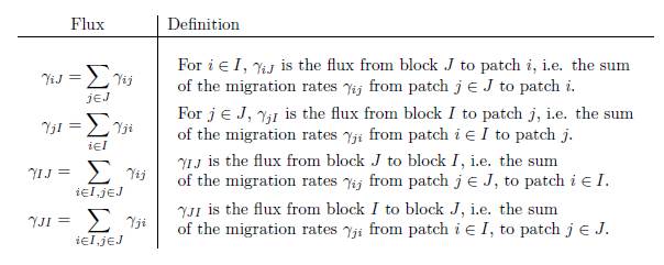
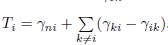
For each patch i ∈ I we denote by γiJ the flux from block J to patch i, and for each patch j ∈ J we denote by γjI the flux from block I to patch j, as defined in Table 1. For each patch i we denote by Ti the sum of all migration rates γji from patch i to another patch j ̸= i (i.e. the outgoing flux of patch i) minus the sum of the migration rates γik from patch k to patch i, where k belongs to the same block as i. Hence, we have:
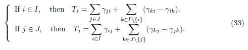
We make the following assumption on the migration rates:
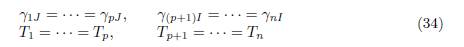
where γiJ , for i ∈ I and γjI , for j ∈ J are defined in Table 1 and Ti are given by (33).
We have the following result:
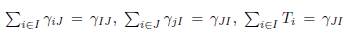
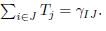
Lemma 4.6. Assume that the conditions (34) are satisfied, then for all i ∈ I and j ∈ I one has

where γIJ and γJI are defined in Table 1.
Proof. The result follows from
 and
and
In the next theorem, we will show that, at the equilibrium, and under certain conditions relating to the migration rates, we can consider the n-patch model as a 2-patch model coupled by migration terms, which are not symmetric in general. Mathematically, we can state our main result as follows:
Theorem 4.7. Assume that the conditions (32) and (34) are satisfied. Then the equilib-rium of (9) is of the form
where (x∗ 1, x∗ n) is the solution of the equations
that is to say, (x∗ 1, x∗ n) is the equilibrium of a 2-patch model, with specific growth rates pr1 and qrn, carrying capacities K1 and Kn and migration rates γJI from patch 1 to patch 2 and γIJ from patch 2 to patch 1.
Proof. Assume that the conditions (32) are satisfied. Then the equilibrium of (9) is the unique positive solution of the set of algebraic equations
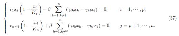
We consider the following set of algebraic equations obtained from (37) by replacing xi = x1 for i = 1 · · · p and xi = xn for i = p + 1 · · · n:
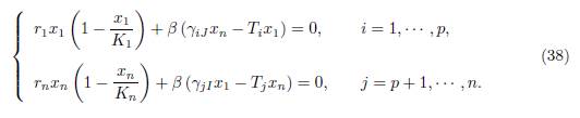
Now, using the assumptions (34), together with the relations (35), we see that the system (38) is equivalent to the set of two algebraic equations:
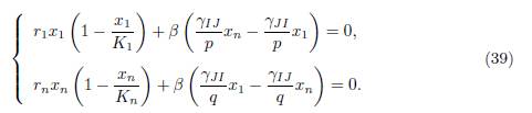
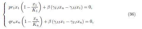
We first notice that if x1 = x∗ 1, xn = x∗ n is a positive solution of (39) then xi = x∗ 1 for i = 1, · · · , p and xj = x∗ n for j = 1, · · · , n is a positive solution of (37). Let us prove that (39) has a unique solution (x∗ 1, x∗ n). Indeed, by multiplying the first equation by p and the second one by q, we deduce that (39) can be written in the form (36).
As a corollary of the previous theorem we obtain the following result which describes the total equilibrium population in the two blocks:
Corollary 4.8. Assume that the conditions (32) and (34) are satisfied. Then the total equilibrium population XT ∗ (β) = px∗ 1(β) + qx∗ n(β) of (9) behaves like the total equilibrium population of the 2-patch model
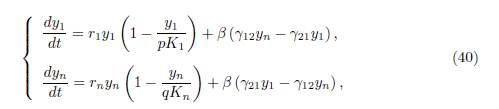
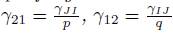
with specific growth rates r1 and rn, carrying capacities pK1 and qKn, and migration rates
 .
.
Proof. From Theorem 4.7, we see that (x∗ 1, x∗ n) is the positive solution of (36). (y1 ∗ = px∗ 1, yn ∗ = qx∗ n) is the solution of the set of equations
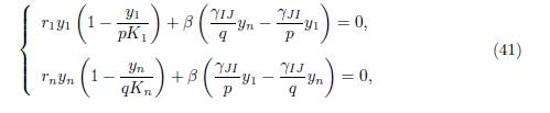
obtained from (36) by changing variables to y1 = px1, yn = qxn. The system (41) has a unique positive solution which is the equilibrium point of the 2-patch model (40).
We can describe when, under the conditions (32) and (34), the migration pattern is beneficial or detrimental in Model (9).
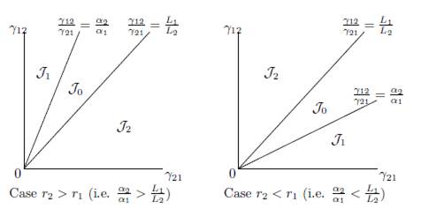
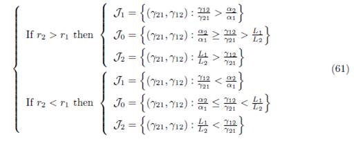
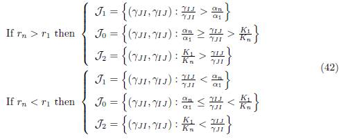
We consider the regions in the set of parameters γIJ and γJI , denoted J0, J1 and J2, depicted in Figure 1 and defined by:
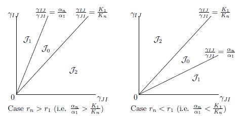
Figure 1 Qualitative properties of Model (9) under the conditions (32) and (34). In J0, fragmentation benefits the total equilibrium population. This effect is detrimental in J2. In J1, the effect is beneficial for β < β0 and detrimental for β > β0.
where α1 = r1/K1 and αn = rn/Kn.
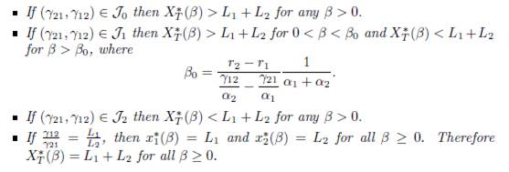
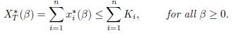
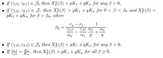
Proposition 4.9. Assume that the conditions (32) and (34) are satisfied. Then the total equilibrium population XT ∗ (β) = px∗ 1(β) + qx∗ n(β) of (9) satisfies the following properties
If r1 = rn then XT ∗ (β) < pK1 + qKn for all β > 0.
If rn # r1, let J0, J1 and J2, be defined by (42). Then we have:
Proof. This is a consequence of Proposition A.1 and Corollary 4.8.
Let us explain the result of Proposition 4.9 in the particular case where p = n − 1. In this case, the condition (34) becomes

where
 . Therefore, if the matrix Γ is symmetric, the conditions (43) are equivalent to the conditions γn1 = . . . = γn,n−1, which mean that the fluxes of migration between the n-th patch and all n − 1 identical patches are equal. Hence, Proposition 4.9, showing that the n-patch model behaves like a 2-patch model, is the same as [12, Proposition 3.4], where the model (9) was considered with Γ symmetric, n − 1 patches are identical and the fluxes of migration between the n-th patch and all these n − 1 identical patches are equal. Thus Proposition 4.9 generalizes Proposition 3.4 of [12], to asymmetric dispersal and for any two identical blocks, provided that the conditions (34) are satisfied.
5. Links between SIS and logistic patch models
5.1. The SIS patch model
In [15], Gao studied the following SIS patch model in an environment of n patches connected by human migration:
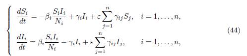
where Si and Ii are the number of susceptible and infected, in patch i, respectively; Ni = Si + Ii denotes the total population in patch i. The parameters βi and γi are positive transmission and recovery rates, respectively. The matrix Γ = (γij) satisfies (3) and describes the movement between patches. The coefficient ε quantifies the diffusion, as our β in (9).
Using the variables Ni, Ii, i = 1, . . . , n, the system (44) has a cascade structure
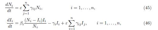
Therefore the infected populations Ii are the solutions of the non-autonomous system of differential equations
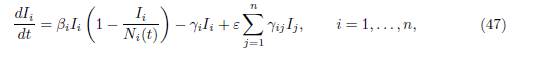
where the total populations Ni(t) are the solutions of the system (45). Hence, the autonomous 2n-dimensional system (44), is equivalent to the family of n-dimensional non-autonomous systems (47), indexed by the solutions Ni(t) of (45). Note that since the γij verify the property (3), the total population is constant: Σn i=1 Ni(t) = N, where N := Σn i=1 (Si(0) + Ii(0)). If the matrix Γ = (γij) is irreducible, then Ni(t), the total population in patch i, converges towards the limit
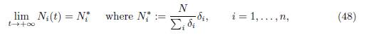
where δ = (δ1, . . . , δn)T is a positive vector which generates the vector space ker Γ. Therefore, (47) is an asymptotically autonomous system, whose limit system is obtained by replacing Ni(t) in (47), by their limits Ni ∗, given by (48):
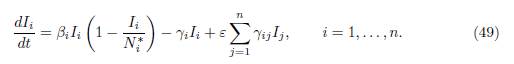
The main problem for (44) is to determine the condition under which the disease free equilibrium, corresponding to the equilibrium I = 0 of (49), is GAS, or the endemic equilibrium, corresponding to the positive equilibrium of (49), is GAS. It is known, see [15, Theorem 2.1], that the disease free equilibrium is GAS if ℛ0 ≤ 1, and there exists a unique endemic equilibrium, which is GAS, if ℛ0 > 1. Here ℛ0 is the basic reproduction number of the model (44), defined as:

A reference work on the basic reproduction number for metapopulations is Arino [3], whereas Castillo-Garsow and Castillo-Chavez [7] and van den Driessche and Watmough [29] give a more general account of the subject.
5.2. Comparisons between the results on (9) and the results on (49)
Gao [15] gave many interesting results on the effect of population dispersal on total infection size. Our aim is to discuss some of the links between his results and the results of the present paper. We focus on two results on the total infection size Tn(ε) = Σn i=1 Ii∗(ε), where (I1 ∗(ε), . . . , In ∗(ε)) is the positive equilibrium of (49). We consider the results of Gao [15] on Tn(+∞) and Tn ′(0).
Proposition 5.1 ([15, Theorem 3.3], [15, Theorem 3.5]). If ℛ 0(+∞) > 1, then

If βi # γi for all i, then
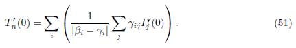
It is worth noting that the formulas (50) and (51) involve the system (49). An important property of this system is given in the following remark.
Remark 5.2. Let N∗ = (N1 ∗, . . . , Nn ∗)T be the vector of the carrying capacities in the system (49). One has N∗ ∈ ker Γ, as shown by (48).
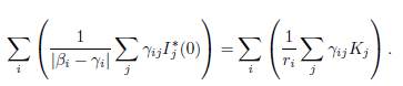
Our aim is to compare the results given by the formulas (50) and (51) when γi → 0, to our results, for the system
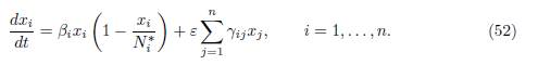
Note that the system (49) reduces to (52) when γi = 0 for all i. More precisely we show that, as γi → 0, the formulas (50) and (51) are the same as the results predicted by Proposition 3.4 and Proposition 4.4.
Proposition 5.3. Let Tn(ε) be the total infection size of (49). Let X∗ T (ε) be the total population size of (52). One has

Proof. When γi → 0 for all i, one has ℛ 0(+∞) → +∞ and Ii ∗(0) → Ni ∗. Therefore, from (50) and (51) it is deduced that
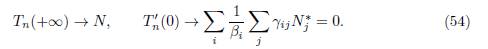
Using the property N∗ ∈ ker Γ, from Proposition 3.4 and Proposition 4.4, it is deduced that:
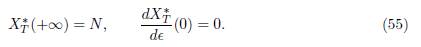
From (54) and (55) we deduce (53).
Actually as shown in Proposition 4.5, we have the stronger result XT ∗ (β) = N for all β≥ 0. But our aim here was only the comparison between (54) and (55).
As shown in Proposition 5.2, the results of Gao [15] on the logistic patch model (49) yield results on the logistic patch model (52) by taking the limit γi → 0. However, the scope of this approach is weakened by the fact that it only applies to the logistic model (52), for which the vector of carrying capacities satisfies N∗ ∈ ker Γ, see Remark 5.2. But this property is not true in general for our system (9), where the condition K ∈ ker Γ does not hold in general.
Our aim in this section is to show that any logistic patch model (9), without the condition K ∈ ker Γ, can be written in the form (49), with the condition N∗ ∈ ker Γ. Indeed we have the following result:
Lemma 5.4. Consider ri > 0, Ki > 0 and Γ as in the system (9). Let δi > 0 be such that (δ1, ..., δn)T ∈ ker Γ. Let N be such that N >
 for i = 1, . . . , n. Let Ni
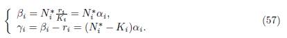
∗ defined by (48). Let βi = ri Ni∗ and γi = βi − ri. Then one has
for i = 1, . . . , n. Let Ni
∗ defined by (48). Let βi = ri Ni∗ and γi = βi − ri. Then one has

Proof. The conditions (56) are satisfied if and only if ri = βi − γi and ri/Ki = βi/Ni ∗. Therefore
To ensure that γi > 0 for all i, just choose N in (48) such that Ni
∗ > Ki for i = 1, . . . , n, that is to say,
 .
.
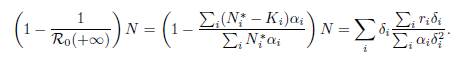
Remark 5.5. According to the change of parameters (57), the logistic patch model (9) can be written in the form of Gao (49), i.e. with the property that N∗ ∈ ker Γ. For the perfect mixing case, the formula (50) and our formula (13) are the same. Indeed replacing βi and γi by (57) in (50), and using (48), we get:
For the derivative, the formula (51) and our formula (28) are the same. Indeed, if we replace βi and γi by (57), in (51), we get:
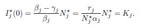
Therefore
The theory of asymptotically autonomous systems answers the question “under which conditions do the solutions of the original 2n-dimensional system (44) have the same asymptotic behavior as those of the n-dimensional limit system (49) ?”. For details and further reading on the theory of asymptotically autonomous systems, the reader is referred to Markus [23] and Thieme [26, 27]. For applications of this theory to epidemic models, see Castillo-Chavez and Thieme [6].
Hence, it is important to know whether or not some of the results of Gao [15] on the SIS model (44) can be deduced from our results on the logistic model (9). It is worth noting that the discussion in this section shows that our results on the logistic patch model imply results on the model (49) and hence, results on the original model 2n-dimensional system (44). However, it is needed that βi > γi for i = 1, . . . , n. Indeed, according to (57), one has ri = βi − γi > 0. On the other hand, the condition βi > γi is not required in all patches of the system (44). Another challenging problem is the study of the model (49), in the general case where N∗ = (N1 ∗, . . . , Nn ∗)T is not necessarily in the kernel of Γ.
6. Three-patch model
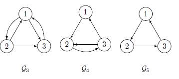
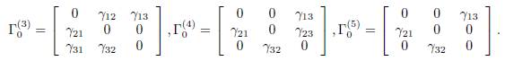
In this section, we consider the model of three patches coupled by asymmetrical terms of migrations. Under the irreducibility hypothesis on the matrix Γ, there are five possible cases, modulo permutation of the three patches, see Figures 2 and 3.
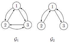
The connectivity matrices associated to the graphs G1 and G2 given by
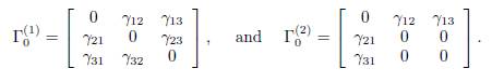
For the remaining cases, the graphs G3, G4 and G5, cannot be symmetrical:
The associated connectivity matrices are given by
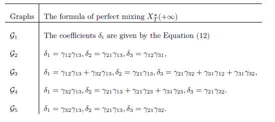
In Table 2, we give the formula of perfect mixing XT ∗ (+∞) for each of the five cases. In the numerical simulations, we show that we can have new behaviors of XT ∗ (β). In the case n = 2, it was shown in [1, 2] that there exists at most one positive value of β such that XT ∗ (β) = K1 + K2. In [12], in the case n = 3 and Γ is symmetric, we gave numerical values for the parameters such that there exists two positive values of β such that XT ∗ (β) = K1 + K2 + K3, and we were not able to find more than two values. The novelty when Γ is not symmetric is that we can find examples with three positive values.
Table 2 The generator δ of ker Γ, for the five cases. The perfect mixing abundance X∗ T (+∞) is computed with Eq. (13).
Indeed, we may have the following situation :
 and X∗
T (+∞) < K1+K2+K3, and there exist three values 0 < β1 < β2 < β3 for which we have
and X∗
T (+∞) < K1+K2+K3, and there exist three values 0 < β1 < β2 < β3 for which we have
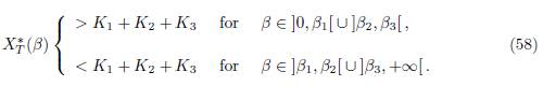
The same situation holds for each of the five graphs G1, G2, G3, G4 and G5, i.e, there exist three values 0 < β1 < β2 < β3 for which (58) hold. See Figures 4, (for the graph G1), 5, (for the graph G2), 6-a, (for the graph G3), 6-b, (for the graph G4), and 6-c, (for the graph G5).
Table 3 The numerical values of the parameters for the logistic growth function and migration coeffi-cients of the model (9), with n = 3, used in Figures 4,5,6-a,6-b and Figure 6-c. For all figures we have(r1, r2, r3, K1, K2, K3) = (4, 0.7, 0.6, 5, 1, 4). The perfect mixing abundance XT ∗ (+∞) is computed with Eq. (13) and the derivative of the total equilibrium population at β = 0 is computed with Eq. (28).
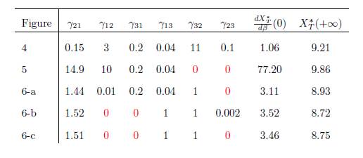
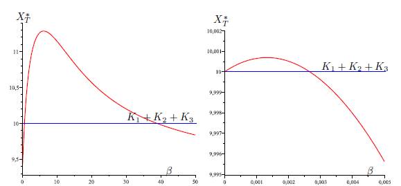
Figure 4 Total equilibrium population XT ∗ of the system (9) (n = 3) as a function of the migration rate β. The figure on the right is a zoom, near the origin, of the figure on the left. The parameter values are given in Table 3.
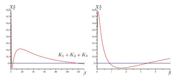
Figure 5 Total equilibrium population XT ∗ of the system (9) (n = 3) as a function of the migration rate β. The figure on the right is a zoom, near the origin, of the figure on the left. The parameter values are given in Table 3.
7. Conclusion
The aim of this paper is to generalize, to a multi-patch model with asymmetric dispersal, the results obtained in [12] for a multi-patch model with symmetric dispersal.
In Section 3 we considered the particular case of perfect mixing, when the migration rate goes to infinity, that is, individuals may travel freely between patches. As in [12], we compute the total equilibrium population in that case, and, by perturbation arguments, we proved that the dynamics in this ideal case provides a good approximation to the case when the migration rate is large. Our results generalize those of [2] (asymmetric migration matrix, only two patches), [10] (arbitrarily many patches, but the migration matrix is symmetric and zero outside the corners and the three main diagonals), and [12] (arbitrarily many patches; arbitrary, but symmetric, migration).
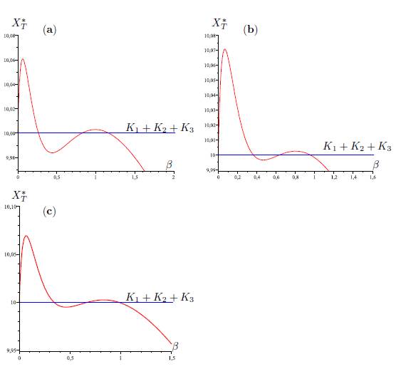
Figure 6 Total equilibrium population XT ∗ of the system (9) (n = 3) as a function of the migration rate β. The parameter values are given in Table 3.
In Section 4 we considered the equation total equilibrium population = sum of the carrying capacities of the patches. (59)
We gave a complete solution in the case when the n patches are partitioned into two blocks of identical patches. Our results mirror those of [2], which deals with the two-patch case. Specifically, Equation (59) admits at most one non-trivial solution.
In Section 5, we consider a SIS patch model and we give the links with the logistic model.
In Section 6 we give numerical values for the dispersion parameters such that Equation (59) has at least three non-trivial solutions. In [12] we proved that for three patches and symmetric dispersal, there may be at least two solutions. A mathematical proof that, when n=3, Equation (59) has at most three solutions, would certainly be desirable, and could spur further work. Upper bounds for arbitrarily many patches would also be interesting.