English (pdf)
 Article in xml format
 Article references
 Send this article by e-mail
 Cited by SciELO
  Cited by Google
  Similars in
SciELO
Similars in
SciELO  Similars in Google
 Permalink
1.The Hilbert transform
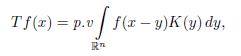
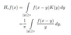
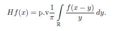
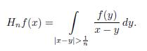
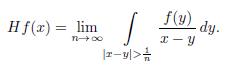
The Hilbert transform of a sufficiently well-behaved function f(x) is defined to be
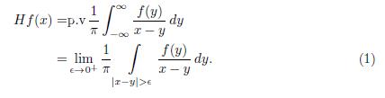
The central idea behind the definition of transform is quite simple, namely to transform f(x) by convolving it with the kernel
The theory of singular integrals has its roots in the works of Calderón and Zygmund [3] and Mihlin [15]. The Hilbert transform is a fundamental example in the theory of singular integrals. Two celebrated results about the boundedness properties of H can be remarked: the Lp-boundedness result of H due to M. Riesz, and the weak-(1; 1) boundedness of H, due to Kolmogorov. For the general aspects of the theory of singular integrals as well as the modern developments about the theory of pseudo-differential operators, which are important generalizations of the singular integrals, we refer the reader to [7, 8, 11, 12, 17]. For a substantial treatment about the subject we refer the reader to [14], and for a concise review on the subject we refer to [9].
This paper is organized as follows. In Section 2 we present some preliminaries dedicated to the rearrangements of functions. In Section 3, we present the definition of Calderón-Zygmund operators and we motivate the Hilbert transform as a fundamental example of this definition. Finally, in Section 4, we make a review of the Lp-boundedness of the Hilbert transform.
2. Preliminaries
Let us begin by presenting some definitions and properties regarding to the decreasing re-arrangement. As usual (ℝ; ℐ; m) stand for the one-dimensional Euclidean space endowed with the Lebesgue measure and F(ℝ; ℐ) denote the set of all ℐ-measurable functions on R.
Definition 2.1. The distribution function Df of a function f 2 F(ℝ; ℐ) is given by

for all λ ≥0.
Observe that the distribution function Df depends only on the absolute value of the function f and its global behavior. Moreover, notice that Df may even assume the value +∞.
It should be pointed out that the notation for the distribution function in (2) is not standard, other authors use the notations f*, μf, df , λf , among others.
The distribution function Df enjoy the following properties.
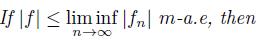
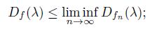
Theorem 2.2. Let f and g be two functions in F(ℝ; L). Then for all λ1; λ 2; λ 3 ≥ 0 we have:
a)Df is decreasing and continuous from the right;
b) |g| ≤ |f| m-a.e implies that Dg(λ) ≤ Df (λ);
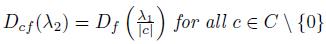
c)
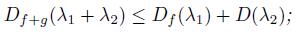
d)
e)
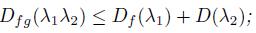
f)
g)
For the proof of all this properties see [6, 5].
With the notation of the distribution function we are ready to introduce the decreasing rearrangement function and its important properties.
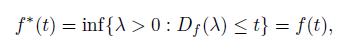
Definition 2.3. Let f 2 F(ℝ; ℐ). The decreasing rearrangement of f is the function
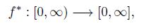
defined by
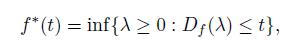
taking the usual convention that inf(
The next theorem establishes some basic properties of the decreasing rearrangement function.
Theorem 2.4. The decreasing rearrangement function has the following properties:
(a) f* is decreasing;
(b) f* (t) > λ if and only if Df (λ) > t;
(c) f and f* are equimeasurable, that is Df (λ) = Df* (λ) for all λ ≥ 0;
(d)
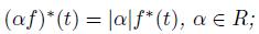
(e)
(f)
(g) For 0 < p < ∞, (|f|p)* (t) = [f* (t)]* ;
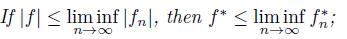
(h) If |f| ≤ |g|, then f*(t) ≤g*(t);
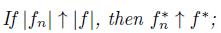
(i)
(j)
 .
.
(k)

For the proof of all these properties see [6, 5]. The next result tells us that a function cannot have two different decreasing rearrangements, see [6] and also [5, Theorem 1.8].
Theorem 2.5. There exists only one right-continuous decreasing function f equimea-surable with f.
For a positive strictly decreasing function f, it is itself its decreasing rearrangement, as the next result shows.
Theorem 2.6. Let f be a strictly decreasing and non-negative function on (0; 1) then f (t) = f(t).
Proof. Consider
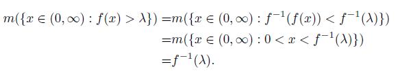
Take t = f -1(λ) then λ= f(t). Thus
that is f (t) = f(t), as we claim. The proof of Theorem 2.6 is complete.
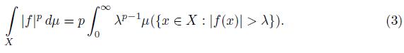
The following theorem is quite important since it allows us to calculate an integral in a general space via an one-dimensional integral. The formula (3) below is sometimes called the Cavalieri principle.
Theorem 2.7. Let (X;
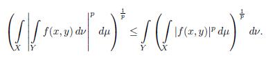
For the proof of this statement we refer to [6]. The next theorem, known as Minkowski integral inequality, will be useful in proving latter results in this paper.
Theorem 2.8 (Minkowski integral inequality). Let (X;
For the proof of this statement see [6]. A function and its decreasing rearrangement has the same Lp-norm. Indeed, we have the following Lp-identity.
Theorem 2.9. Let f Є Lp(ℝ), 1 ≤p < ∞. Then
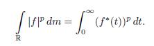
Proof. By Theorem 2.7 and Theorem 2.4 (c), we have that
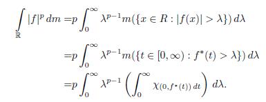
Next, by applying the Fubini theorem, we have that
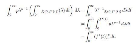
The proof is complete.
The following inequality is due to Hardy and Littlewood.
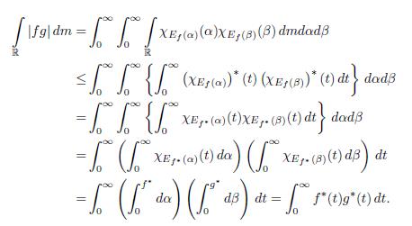
Theorem 2.10. If f and g, both belong to F(ℝ; ℒ), we have the identity
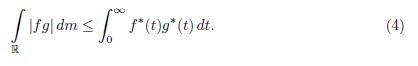
Proof. Assume first that f =xA and g =xB are characteristic functions where A and B are sets in ℒ. We suppose without loss of generality that m(A) and m(B) are finite. Then it follows from Theorem 2.4(i) that
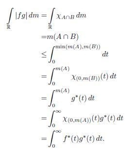
In general let f and g be two functions belonging to F(ℝ; ℒ). Then
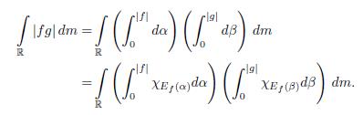
It follows from Fubini’s theorem and Theorem 2.4 (h) and the property (k) of this theorem that
The proof is complete.
Theorem 2.11. Let f Є L1(ℝ). Then
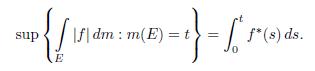
Proof. Given the real number t > 0, we have that
The following is a well known fact from the measure theory: if m(Ef (λ)) > t > 0, then there exists a set E Є ℒ such that E

The proof is complete.
3.Calderon-Zygmund singular integral operators
Taking into account the Calderón-Zygmund theory we are going to have the Hilbert transform as a fundamental example. We recall the following definition.
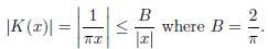
Definition 3.1. Suppose that K(x) 2 Lloc(ℝn
(a)
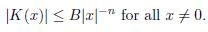
(b)
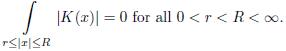
(c)
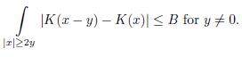
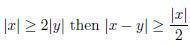
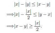
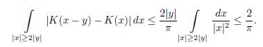
A kernel as in Definition 3.1 is called the Calderón-Zygmund Kernel where B is a constant independent of x and y. The condition (c) is called Hörmander condition..
Now, we present the following fundamental theorem.
Theorem 3.2. Suppose that K is the Calderón-Zygmund kernel. For > 0 and f 2 Lp(ℝn), 1 < p < 1, let
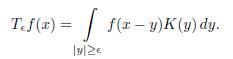
Then the following statements holds:
(1) ||TЄ f||Lp ≤ Ap||f||Lp where Ap is independent of and f.
(2) For any f 2 Lp(ℝn), lim TЄ f exists in the sense of the Lp -norm. That is, there exists an operator T such that
holds for almost every x Є ℝn .
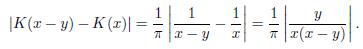
In addition, one can show that K(x) =
(a)
(b)
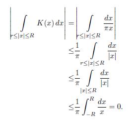
Since
Note that
Now, if
 . Indeed
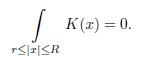
Consequently,
Hence K(x) =
By Theorem 3.2, we have that
So we might say roughly that Hilbert’s transformation of a function f is the convo-lution of f with the Calderón-Zygmund kernel K(x) =
4. A theorem due to E. M. Stein and G. Weiss
This section is based on [1, 4]. The following lemmas will be helpful for the proof of Theorem 4.3. We present these lemmas and their proofs below.
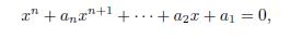
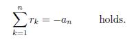
Lemma 4.1. Let P (x) = xn + anxn +1 + + a2x + a1 be polynomial of degree n. Let r1; r2; ; rn be the roots of P (x) = 0, then
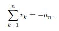
Proof. The proof uses the mathematical induction. When n = 2, the polynomial x2 + α2x + α1 = 0 has two roots, r1 and r2, such that
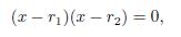
then
In consequence
Hence r1 + r2 = α2. Now, for n = 3, the polynomial x3 + α3x2 + α2x + α1 = 0 has three roots named r1; r2 and r3 such that
From this last equality we have that
Next, suppose that for
the property
Now, the polynomial xn+1 + αn+1xn + + α2x + α1 = 0, has n + 1 roots r1; r2; ; rn+1 such that
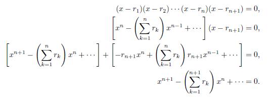
Therefore
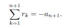
The proof of Lemma 4.1 is complete.
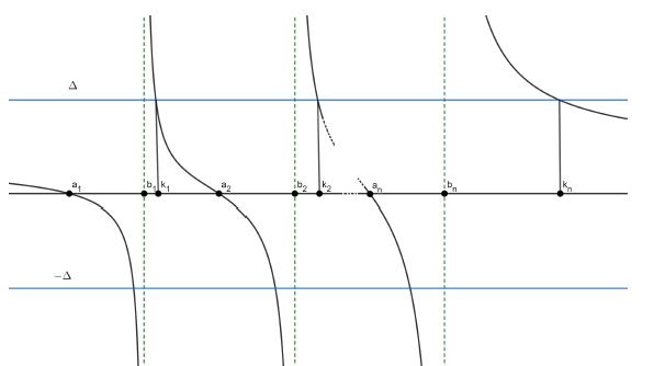
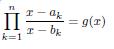
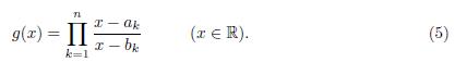
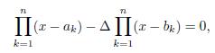
Lemma 4.2. Suppose that αi , bi (i = 1; 2; 3; …, n) are real numbers satisfying that α1 < b1 < α 2 < b2 < … < an < bn and let g be the rational function
If Δ # 1, then the equation g(x) = |Δ| has n different roots r1; r2; ; rn which satisfy that
Furthermore, if Δ > 1, then

Proof. Since g has a simple pole at each bk, (k = 1; 2; 3; …,n) and
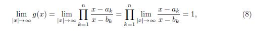
there are exactly n different solutions, say r1; r2; ; rn to the equation g(x) = |Δ| (Δ # 1). Then
For
 , we have that
and so
Where
Then
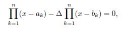
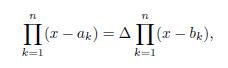
Which implies that
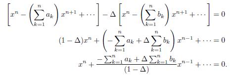
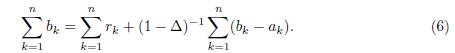
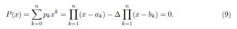
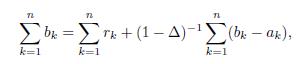
Since r1; r2; ; rn are the roots of the polynomial P (x) = 0, then by Lemma 4.1 we have that
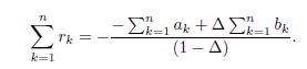
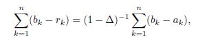
In consequence,
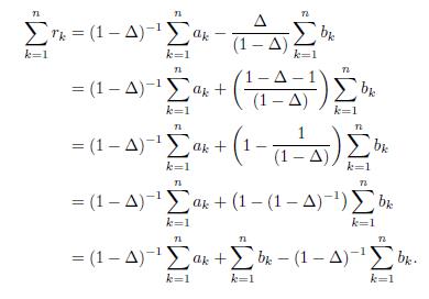
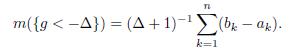
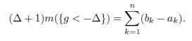
Hence
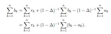
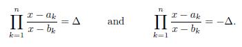
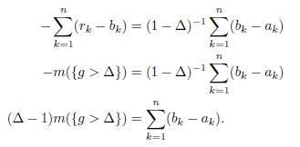
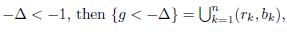
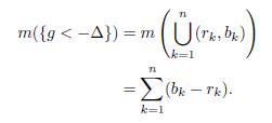
If Δ > 1, then
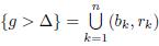 (see figure 1) and so
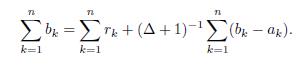
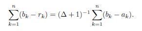
Since
we have that
and putting these equations together we have that
Moreover, if
 (see figure 1). Hence
Now, we have
Also,
In consequence
Finally,
In view of the analysis above, we conclude that

The proof of Lemma 4.2 is complete.
In the following result we can observe that the distribution function of H E depends only on the measure of E and not on the way in which E happens to be distributed over the real line.
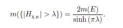
Theorem 4.3 (Stein-Weiss [19]). Let E be the union of finitely many disjoint intervals, each of finite length. Then
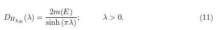
Where DHxE (λ) = m({|HxE| > λ).
Proof. We may express the set E in the form
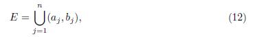
where α1 < b1 < α 2 < b2 < < α n < bn. We already know that
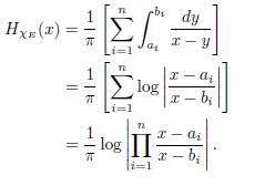
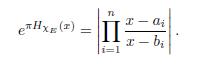
Fix λ > 0, and let F = {|HxE| > λ}. Then m(F ) = DHxE (λ). Since

we have that
If we set
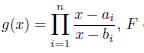 can be decompose as

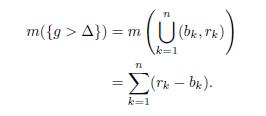
Now, by applying Lemma 4.2 to g we obtain,
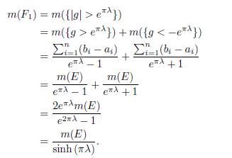
Next, for F2, we have that,
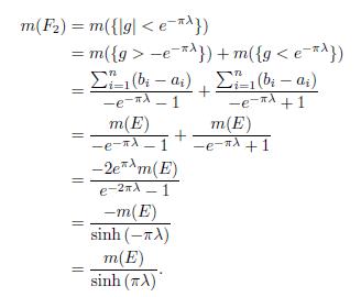
Finally
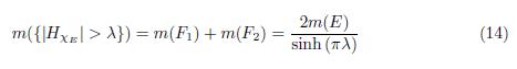
i.e.
The proof of Theorem 4.3 is complete.
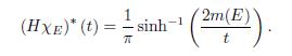
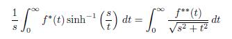
A short proof of the Stein-Weiss theorem using complex-variable methods can be found in Calderón [2] and Garnett [13]. Also, an additional discussion can found in Sagher and Xiang [18]. The Stein-Weiss theorem has been discussed for the ergodic Hilbert transform by Ephremidze [10]. As a corollary of Theorem 4.3, given that f is essentially the inverse function of Df (λ), we compute (HxE)* (t) as follows.
Corollary 4.4. Let E
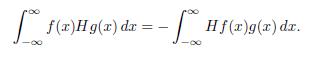
The next theorem shows that the operator H is anticommutative.
Theorem 4.5. Let f Є Lp(ℝ) and g 2 Lq(ℝ) (1 < p < ∞). Then
Proof. Let us start by defining
Note that
Consequently,
An application of Fubini Theorem gives
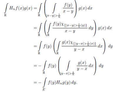
Finally by the monotone convergence Theorem we have that
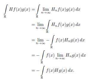
The proof is complete.
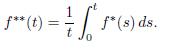
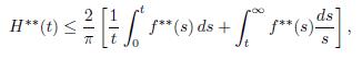
The following result, due to O’Neil, provides a bound of (Hf)** . We provide a proof with enough details.
Theorem 4.6 (O’Neil-Weiss [16]).
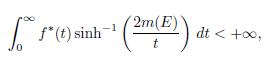
The function Hf(x) exists almost everywhere and for each s > 0 one has that
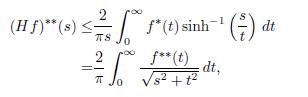
where
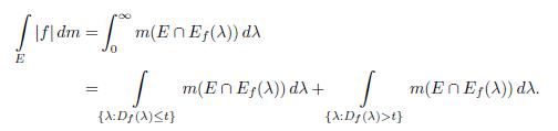
Proof. By Theorem 2.11, the statement will be established if we can show
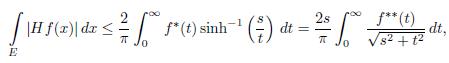
for each set E of measure s, that is m(E) = s.
Given such a set, let E1
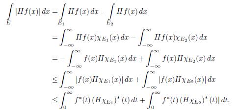
By Corollary 4.4, the previous expression is equal to
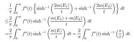
So the desired inequality holds. The equality
follows by integration by parts. The proof of Theorem 4.6 is complete.
Corollary 4.7 (O’Neil-Weiss’s Inequality). Let f be a measurable function on (-∞;∞). Then
for each t > 0.
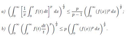
We shall need the following form of the Hardy inequality (see [6]).
Lemma 4.8. If p > 1 and f is a nonnegative function defined on (0, ∞). Then:
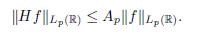
Now we present a theorem due to M. Riesz.
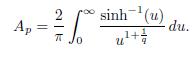
Theorem 4.9 (M. Riesz Theorem). If 1 < p < ∞ and f Є Lp(ℝ). Then there exists Ap independent of f 2 Lp(ℝ) such that
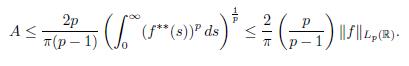
Proof. By Corollary 4.7 we have that
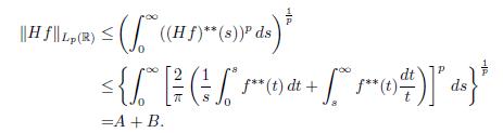
Now, by Lemma 4.8(a), we have that
And by part (b) of Lemma 4.8 we have that
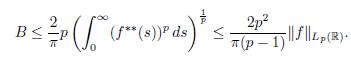
The analysis above shows the theorem.
We can also give another proof of Theorem 4.9 using Minkowski’s integral inequality, as it is shown below. The proof is due to O’Neil-Weiss [16].
Proof. By making an appropriate change of variables and by employing Minkowski’s integral inequality (see Theorem 2.8), we have that
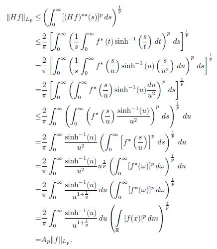
Thus we proved Theorem 4.9 with