


Servicios Personalizados
Revista
Articulo
 Inglés (pdf)
 Articulo en XML
 Referencias del artículo
 Enviar articulo por email
Indicadores
-
 Citado por SciELO
 -
 Accesos
Links relacionados
-
 Citado por Google
 -
 Similares en
SciELO
Similares en
SciELO -
 Similares en Google
Compartir

 Permalink
Ensayos sobre POLÍTICA ECONÓMICA
versión impresa ISSN 0120-4483
Ens. polit. econ. vol.29 no.66 Bogotá jul./dic. 2011
OVERCOMING THE FORECASTING LIMITATIONS OF FORWARD-LOOKING THEORY BASED MODELS
SUPERANDO LOS LÍMITES PREDICTIVOS DE LOS MODELOS BASADOS EN LA TEORÍA CON VISIÓN DE FUTURO*
SUPERANDO OS LIMITES PREDITIVO DOS MODELOS BASEADOS NA TEORIA COM VISÃO DE FUTURO
Andrés González
Lavan Mahadeva
Diego Rodríguez
Luis Rojas
*Este artículo expresa exclusivamente las opiniones de los autores y no las del Banco de la República ni de su Junta Directiva.
Los autores son respectivamente: director, Departamento de Modelos Macroeconómicos del Banco de la República; Senior Research Fellow, Oxford Institute for Energy Studies, Oxford University; jefe de Modelos Macroeconómicos, Departamento de Modelos Macroeconómicos del Banco de la República y estudiante del Doctorado en Economía del European University Institute.
Correo electrónico: agonzago@banrep.gov.co
Documento recibido: 25 de mayo de 2011; version final aceptada: 8 de noviembre de 2011.
Los modelos teóricamente consistentes deben mantenerse modestos para ser útiles. Si su fin es pronosticar eficazmente, tienen que basarse en datos ruidosos, irregulares, no modelados y que se traten del futuro. Los agentes también pueden usar estos datos para formular sus propias expectativas. En este artículo ilustramos un esquema para condicionar de manera simultánea los pronósticos y expectativas internas de los modelos DSGE lineales con visión de futuro, con los datos a través de un filtro de Kalman de intervalos fijos suavizado.
También ensayamos con algunos diagnósticos de este método; específicamente, las descomposiciones que revelan cuando una predicción condicionada sobre un juego de variables implica los cálculos de otras variables que son inconsistentes con los precedentes económicos.
Clasificación JEL: F47, E01, C61.
Palabras clave: predicción condicional, DSGE, filtro de Kalman.
Theory-consistent models have to be kept small to be tractable. If they are to forecast well, they have to condition on data that are unmodelled, noisy, patchy and about the future. Agents can also use these data to form their own expectations. In this paper we illustrate a scheme for jointly conditioning the forecasts and internal expectations of linearised forward-looking DSGE models on data through a Kalman Filter fixed-interval smoother. We also trial some diagnostics of this approach, in particular decompositions that reveal when a forecast conditioned on one set of variables implies estimates of other variables which are inconsistent with economic priors.
JEL classification: F47, E01, C61.
Keywords: Conditional forecast, DSGE, Kalman filter filter.
Os modelos teoricamente consistentes devem ser mantidos modestos para serem úteis. Se a sua finalidade é prognosticar eficazmente, eles têm que estar baseados em dados barulhentos, irregulares, não modelados e que se refiram ao futuro. Os agentes também podem utilizar estes dados para formular as suas próprias expectativas. Neste artigo, ilustramos um esquema para condicionar, de maneira simultânea, os prognósticos e expectativas internas dos modelos DSGE lineares com visão de futuro, com os dados através de um filtro de Kalman de intervalos fixos suavizado. Também tentamos com alguns diagnósticos deste método; especificamente, as decomposições que revelam quando uma predição condicionada sobre um jogo de variáveis implica os cálculos de outras variáveis que são inconsistentes com os precedentes econômicos.
Classificação JEL: F47, E01, C61.
Palavras-chave: Predição condicional, DSGE, filtro de Kalman.
I. INTRODUCTION
Forecasting is a very different exercise from simulating, especially when forecasts are used to guide and explain policy. A policy forecast should relate to all the data that features in the public debate, even if that comes in an awkward variety of shapes and forms. After all, agents in the real world could also be reacting to this data, after taking account of their measurement error.
The need to reach out and connect with the relevant data is especially important when the forecast is based on a dynamic stochastic general equilibrium (henceforth, DSGE) model. DSGE models are distinguished by having a greater theoretical input. Indeed, this explains their appeal to policy; with more theory it is easier to use the forecast as a basis for discussion and explanation. Yet, more theory often comes at a cost in terms of worse forecast performance because it is harder to match more rigid theoretical concepts to available data and extending the model comes at great cost. But, if any policy model ultimately does not link to the real world, it cannot be of much use as a policy tool.
There are two broad categories of reasons why we should expect the useful data set for a policy forecast to be awkward:
1) Real world data is unbalanced.
a) Real world data comes with different release lags: we have more up to date information on some series than on other series.
b) Real world data comes with different frequencies. Some relevant economic information is only available annually whilst some is in real time.
c) There may be useful off-model information on the expected current and future values of exogenous and endogenous variables from other sources which cannot be incorporated into the model system, at least not without making the model cumbersome. Sometimes this information is patchy: we have information on values at some future point. But sometimes the information may be complete for the whole horizon, as would be the case if we use the forecasts from other sources for the exogenous variables.
2) Real world data is subject to time-varying measurement uncertainty. This also has many aspects.
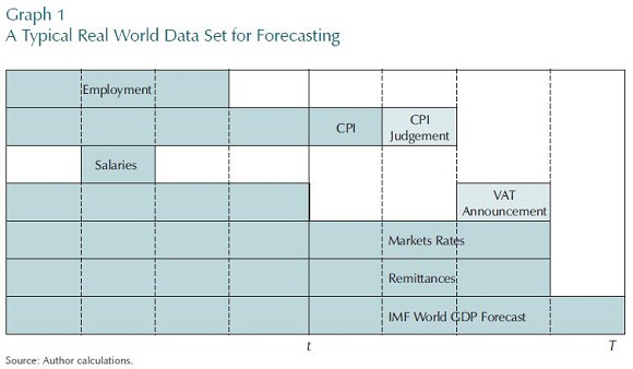
Graph 1 shows us some examples of the kind of awkward data that one can expect to deal with in the real world. Assume we are time t and planning to forecast up until time T.a) Real world data is imperfectly measured. For this reason published data are often revised.
b) Real world data that is available to agents may differ from the economic concept that matters to their decisions.
c) Forecasts from other models and judgement also come with a measurement error.
• First, we have series, such as employment, which come to us after a longer delay.
• In contrast, series such as CPI are very up to date. And then, often it is the case that a combination of small monthly models —monthly data on some prices
and even information from the institutions which set regulated prices— can give a decent forecast of consumer prices into the next quarter.
• Some data is only available annually. For example, in Colombia the only national salary series can be constructed from the income side of annual national accounts.
• Then, there is information on what can happen quite far ahead. The government can preannounce its VAT plans which will have a first-round effect on
inflation. In monetary policy conditioning scenarios, the central bank credibly announces its interest path (Laséen and Svensson, 2011).
• Also, we have implied forecasts from financial markets data. For example, removing risk premia and other irrelevant effects from a yield curve gives us data on what the risk-free expectation of future interest rates may be. Some other important special cases of this type of information would be world interest rates, world commodity prices and expected monetary policy rates. The forecast should then be conditioned on the useful information contained in this data.
• Finally, there are forecasts from other models. A good example is that of remittances. Using information on migration trends, exchange rate movements, and some disaggregated capital flow data, a specialist can come up with a good forecast for remittances, or at least a forecast that is better than one that a DSGE model can generate internally. Population growth and relative food prices are two other examples of variables that might also be best forecast separately. Similarly, forecasts for the GDP of important trading partners should probably come from forecasters in those countries or from
international institutions, such as the IMF, which are more capable of forecasting those series.
The contention of this paper is that a model can only provide both decent predictions and useful explanations if it takes account of the real world data set. Obviously, if there is valuable information is in this awkward data set then the better forecasts should not ignore it. But more subtly, if the agents whose behaviour we are trying to model might be using this type of information when they form expectations, we would also need to mimic them if we are to expect to pick up their behaviour. For example, if the data is noisy and is infected by short-term movements which have nothing to do with the fundamentals, agents will ignore some of the movements in the data.. So, then should the forecast also do so.
Through the method described in this paper, a forecast can bring this rich but awkward information to bear in forming a policy forecast with a forward-looking DSGE model. The basic idea is to first solve the model for rational expectations under the assumption that the data up until the end of the forecast horizon is perfectly known. Then, in a second stage, the data uncertainty problem is wrapped around these solutions which are the state equations of a Kalman filter. In Kalman filter terminology, the solution is fixed-interval smoothing.
This method has advantages over existing strategies.
First it allows for measurement error of future data. If that future data consists of forecasts produced by other models, then this model's forecast should take account of the external models' errors. If that future data were instead announcements or plans made by external institutions, this method allows for the important possibility of imperfect credibility by incorporating that as measurement error. For example, a preannounced tax change may not be fully credible.
Another important special case is financial market data. Financial market data is noisy in the sense that the price that data measures diverges from the economic concept that matters to agents. If agents have a longer holding horizon than financial market participants, they would not react to short-term, reversible, movements in financial data. Not to adjust for this would mean that forecasts might bounce around with financial data unrealistically. An influential paper by Lettau and Ludvigson (2004) emphasises that movements in short-term financial market data will be smoothed by agents, and this should also matter when policy modelers assess their impact on macroeconomic variables.
Policy forecasters commonly smooth financial market data by imposing prior views on the initial values and forecasts of financial variables; these are the controversial constant exchange rate and interest rate assumptions. Economic shocks are then made endogenous to make the model's solutions comply with those priors. Our proposal is an alternative way of attaining the same result, and one which does not involve our rewriting the economic model to make structural shocks endogenous, for now those deviations are classified as data noise terms.
A second advantage of this method is that the model does not need to be rewritten each time the shape of the data of each given series changes. One only has to fill the parts of the data set where data exists and put blanks (NAs!) in where there is nothing available. With this method, one can imagine how the task of building the data set and that of maintaining the forecasting model can become separate and hence, carried out at different intervals and by different groups of specialists.
Third, we can be much more imaginative with what data we use with this method. In this paper, we show how the measurement equations can be adapted to push the forecast towards where there is interesting information without having to extend the economic part of the model. In this way, we can exploit the interesting information in money data without making that part of the endogenous core of the model, for example. We can allow for the peculiarities of the national accounts data, and especially what we know about its revisions policy. We can bring in information from surveys that we know are important in monetary policy decisions.
Another advantage to this approach is that it allows us access to the whole toolkit that comes with the Kalman filter. We show how we can derive decompositions of forecasts according to the contributions of data, and not just according to the contributions of economic shocks, as is standard. In fact, we can show how estimates of the contributions of the shocks depend on data. Going further, we also show how we can try and spot where forecasts will not be well identified in terms of shocks. The information context of different series to the forecast can be measured. And then retrospectively, we can use this technology to compare the forecasts across different vintages of data to see if policy mistakes were due to data mismeasurement, as suggested by Orphanides (2001) and Boragan Aruoba (2004). This means that we can present the differences between forecasts across policy rounds in terms of the contribution of news in the data. This incremental way of presenting the forecast to a busy Monetary Policy Committee is at least more efficient. All these outputs help us to integrate the model's forecast into the central bank's policy decisions.
This paper belongs to a branch of the forecasting literature that addresses the problem that it is simply not viable for one model to incorporate all useful information. An important paper by Kalchbrenner, Tins-ley, Berry, and Garrett (1977) formalises how to bring in auxiliary information of a different frequency and with patchy observations into a backward-looking forecasting model —model-pooling. Papers by Leeper and Zha (2003) and more recently Robertson, Tallman, and Whiteman (2005) and Andersson, Palmqvist, and Waggoner (2010) have implemented conditioning in VAR models. Working with a forward-looking DSGE model, Monti (2010) demonstrates how to pool the model forecast with judgemental forecasts, and Beneš, Binning, and Lees (2008) present tests of how plausible these pooled forecasts are. Schorfheide, et al., (2011) discusses appending forecasts for non-modelled variables onto a DSGE model. But these papers do not consider how the agents in the DSGE model might themselves be using future information.
This crucial step was taken in a recent paper by Maih (2010) —the closest to our work. Maih allows for agents to incorporate future uncertain data in forming expectations and considers the choice between conditioning on future information in the form of a truncated normal distribution which, having upper and lower bounds as well as a covariance and a mean as parameters, is a more general model of conditioning than ours. However, as the variance of a truncated normal variable is a nonlinear function of the bounds, the reader may prefer an approach in terms of means and variances only. Maih did not discuss ways to get around the potentially serious computational costs of solving a forward-looking model with anticipated future data, nor did he discuss unbalanced data. We cover these gaps. We also derive and trial some revealing outputs and diagnostics, new to the conditioning literature.
A systematic conditioning strategy is already common practice among those central banks that pioneered the use of DSGE models to forecast, in Norway, for example.
We acknowledge their contribution without being able to cite unpublished work.
The rest of this paper is organized as follows. Section II summarises our key assumptions and clarifies our notation. Section III presents the solved economic model in the absence of data uncertainty, in this section this is also extended to allow for future data. In Section IV, this is extended to introduce the data into our forecast. Section V discusses the different strategies for modelling data uncertainty. Section VI presents several useful different ways of presenting the policy forecast. Section VII allows for reporting variables. Section VIII discusses the problem of state identification.
Section IX presents some forecasts using this strategy on Colombian data. Section X concludes.
II. THE KEY ASSUMPTIONS, THE SEQUENCING OF SOLUTIONS AND NOTATION
A. CRUCIAL ASSUMPTIONS
The input of this paper is the outcome of a micro-founded general equilibrium problem. We assume that in a prior stage, the relevant decisions of agents have been formulated as optimizing problems, that the first and second-order conditions have been derived and that those conditions have then been aggregated to match the data and transformed into a linear dynamic system with all variables only in terms of log deviations from time-invariant steady-state values. See for example Uhlig (1995). This paper begins at the next stage: where we need to solve to model and then to match it to available data. By solving the model, we mean that we need to model how the monetary policymakers choose their policy instrument and how agents form rational expectations. By forecasting, we mean how we want to use this model to fit and predict available data. We want all these decisions to reflect what data are really available. Even then, as we shall now see, we make use of a separation theorem to focus on the data part of the solution, assuming that the model has been solved and is given to us in a standard form.
B. THE SEQUENCE OF EVENTS AND THE INFORMATION SETS
The choices of policymakers and agents happen at a current time s = t which lies in between 1 and the end of the forecast horizon, T = t + k. Unlike conventional expositions, it is assumed that the potential data set that was available to agents and policymakers at any time in the past up until now, that is at time u (u = 1,..., t), could have included possibly useful off-model information on variables timed from 1 to u + k, and also could have included information about data uncertainty. Later on, we specify exactly what are in the data sets, but here, we just mention that they could contain values of future variables which we interpret as forecasts from other models. As we move from the past to the current date, information is never forgotten. The information sets are written as F0,..., Ft with the property that  for any i < j. The macroeconomic forecaster makes his/her optimal forecasts based on the same data set as the one used by economic agents.
In this set up, the information set is common, the dynamic model linear, the objective function quadratic and expectations rational. Then, the literature on optimal policy under data uncertainty tells us that there is a separation property such that the problem can be split into two artificial stages and solved recursively1.The first stage, where the rational expectations of agents are solved for, is certainty equivalent; at this point, the second-order properties of the data measurement and economic shocks do not matter. Our scheme allows for future data. For that reason, agents and the forecaster must be allowed to see shocks k periods in advance in this artificial first stage, as in Schmitt-Grohé and Uribe (2008). In a second stage, this partial solution is combined with a description of the data and the second-order properties of the data measurement and economic shocks to give the final solution.
C. NOTATION
The operator Ei means that we are taking expectations of a variable with respect to an information set Fi of timing i. Matrices and vectors are in bold, with matrices in upper case. IM refers to the  identity matrix. 0MN is an
  matrix with zero elements.
 refers to the trace of matrix
  refers to the transpose of a matrix
  refers to the Moore Penrose inverse of the matrix
  is the ijth element of the matrix
  .
.
III. SOLVING THE MODEL WITH FUTURE DATA
Incorporating future information substantially expands the number of variables in the model. The purpose of this section is to show how future information can be incorporated into a DSGE model solution without adding substantially to the computational cost, because we only need to carry out some of the less intensive computations on the extended model. Essentially, the solution with future information can be carried by the commonplace solution without future information.
Our starting point is a micro founded general equilibrium problem that has already been expressed in terms of log-linearised deviations from a steady state. The exposition and method of solution follows Klein (2000) closely:

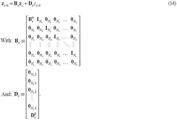
There are N variables in the vector X0s. X0s includes all economic variables endogenous for the model. The Nε variables in Z0s are a set of exogenous variables that follow univariate first-order process. We call them economic shocks. Then there is a matrix equation

where B0ε and D0ε are both diagonal matrices, although B0ε may have a zero entry on its diagonal. These exogenous variables could be extended to include those which follow a VAR but for ease of exposition, and without any loss of generality, here we assume that they are only univariate.
Being exogenous, these variables have no expectational error. Any autoregressive component of the shock is captured in the process (2) such that εs+1 is a martingale difference process with respect to the information set at time s. In particular

and, without loss of generality:

The trivial steady-state solution, defined by X0s = 0N,1and εs= 0Nε,1, for all time s, exists and is unique. The model begins at that steady state:

Then, if we include the variables in Z0s in the vector X0s the solved model can be presented in the form:

The solution in the form of equation (6) can be written in partitioned form, with the exogenous variables  recovered in the lower partition:
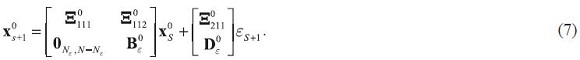
where the matrices B0ε and D0ε are defined in equation (2).
In fact Klein (2000, pages 1417-1418, equations (5.20) and (5.21)) shows that the upper partition of the equation (7) can be partitioned further, where the upper positions of the vector are assigned to the non-predetermined variables, and the lower to the predetermined endogenous variables. From now on it is assumed that the vector X0s is arranged in that way, and Np is defined as the number of endogenous predetermined variables. A variable is predetermined if its generating process is backward-looking, following Klein's definition of a backward-looking process. We need not impose this prior designationbut if not, we would have to allow for more initial conditions for state variables (Sims, 2002), complicating the exposition.
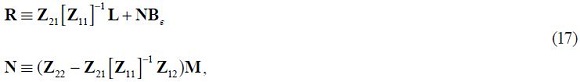
According to this further partition:
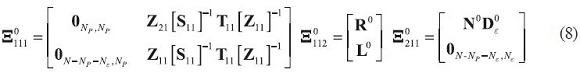
Where:
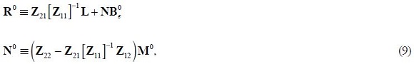
And:

The matrices Sij, Tij, Z  is independent of the parameters of the exogenous shock processes (of matrices B0ε and D0ε).
The matrices  ,
,  and
and  do depend on B0ε and D0ε however.
To allow for the possibility of future data to affect current behaviour, agents must be able to anticipate shocks up until the forecast horizon. In this section, the model and solution is extended to allow for that possibility along the lines of Schmitt-Grohé and Uribe (2008).
It has been assumed that at each time u when a forecast is made, shocks in principle can be anticipated k periods ahead .
. ![]() is defined as perfect information on the vector of shocks εs+1 but known earlier at time s – i for i =0, ..., k – 1. Then, the extended vector of exogenous shocks can be written as:
is defined as perfect information on the vector of shocks εs+1 but known earlier at time s – i for i =0, ..., k – 1. Then, the extended vector of exogenous shocks can be written as:

and the extended vector of economic variables becomes:

The extended system of exogenous variables is now:
It immediately follows that the solution to the extended system is of the form:
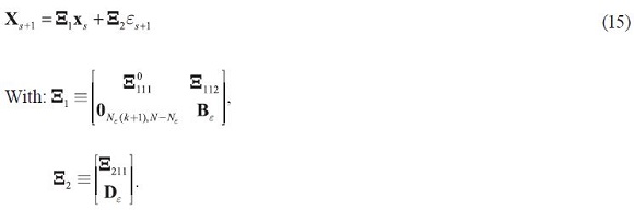
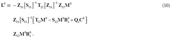
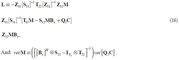
Comparing the two solutions, we can see that only the matrices and need to be recalculated. These matrices can be derived from applying the same formulae as in the model without future shocks, (17), (18) and 3 but when B0ε is replaced with Bε , D0ε is replaced with Dε and C is replaced with 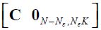 .
.
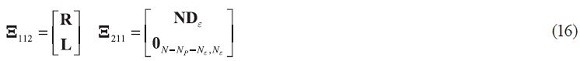
Where:
We have shown that extending the model to incorporate future information does not require carrying out a new Schur factorization on a system with many more endogenous
variables reflecting information on each future period on each variable.
The computational cost would also be high if the vectorised formula 3 were actually used in the larger extended model. Luckily, as Klein (2000) explains, there is an alternative recursive method for calculating M, that can be applied to the extended system to keep the computational cost manageable. In summary, the solution to the model with future shocks can be carried most of the way by the solution to the model without future shocks.
IV. ALLOWING FOR AWKWARD FEATURES OF THE POLICY FORECASTING DATA SET
Up until now, the solution has abstracted from the data set. In this section, the data are introduced. Data can be uncertain and unbalanced. The idea is to wrap the system of (15) around an observation system which relates the true values to the noisy observed data values. We will now describe the observation system.
A. INTRODUCING THE DATA SET
Let the vector yus of size  be the observed data that pertains to variables at time s available in information set u. There can be holes in this data: some observations may not be available at the time s in information set of time u. Thus
  where NDmax is the maximum number of data series possibly available.
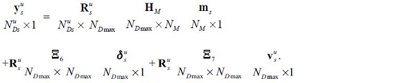
This measurement system is written as:
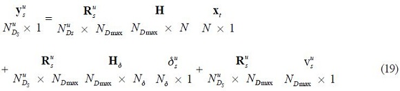
With:
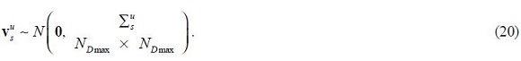
 is the vector of deterministic variables such as dummies, constants or trends which can affect data measurement. (Economic adjustments to the model are already incorporated in the states). Vus is the normally distributed stochastic component of the data errors which have variance-covariance matrices
  that vary both with the time of the data and also with the information set.
Note that the data errors are assumed to be independent of the economic shocks. This assumption is contestable: in many cases, one would expect data measurement problems to be related to the economic cycle or the entry or exit of members of the sample during booms and recessions2. It can easily be relaxed in the Kalman filter algorithms. However, the greater generality makes it harder to identify shocks. And so, the possibly strong restriction that the economic and data uncertainty shocks are independent is imposed in order to avoid getting embroiled in identification problems at this point. Problems of identification are discussed later on.
Rus is a selector matrix which alters the number of rows to suit the number of series with time s data observations within the time u information set: s = 1,...,T and u = 1,..., t. It is assumed that there is data available in principle from time 0 to time T, where T is the end of the forecast, but this is quite general as Rus can fill in the holes.Then, the selector matrices Rus are formed by taking the  identity matrix and deleting rows corresponding to when there are no data series available at time s within information set u.
Naturally, then:

With being a mythical data set where the maximum number of data series is always available (although with measurement error).
That the variance-covariance matrices of the data error are both time and information set heteroscedastic means that available data can be weighted according to how reliable that data is thought to be, but also in real time; that is, relative to when decisions are made and expectations formed.
B. THE INFORMATION SET
The information sets available to agents, policymakers and the forecasters alike at time u is given by:

for u = 1,...,t, t + k = T and  . This structure satisfies the descriptions given in section II.B. As shall be seen shortly, the information set up allows for a data set with the particular characteristics mentioned in the introduction.
C. THE SOLUTION TO THE DATA UNCERTAINTY PROBLEM
The idea is to derive the expectations and forecasts of the economic variables in the model as the fixed-interval smoothed state estimates of the economic system (6) conditional on the measurement system (19) and (20) and the information structure (22).
Although the exposition of the Kalman filter is standard, see Harvey (1991); Durbin and Koopman (2001) for example, it is worth repeating here so that we can clarify our particular notation. Given assumptions that the residuals are Gaussian, the Kalman filter produces the minimum mean squared linear estimator of the state vector xt +1 using the set of observations for time t in information set Fu. Let us call that estimate  and its associated covariance
  . The series of these estimates are a building block towards what we are really interested in: the fixed interval smoothed estimates. We carry out this calculation for each information set, although typically we will only be interested in the forecasts from the last (the current) time u = t information set.
Begin with the initial values contained in information set F1. Then the recursion runs from s = 1 to s = T – 1 over:

Where:
And the  gain matrices are:

the  covariance matrices of one-step estimation error are given by the Riccati equation:

and the  covariance matrices of the one-step-ahead prediction errors in the observation data Lus are defined as:

The initial values are given as:
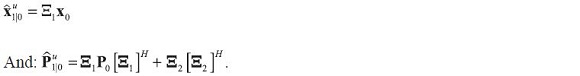
We also need an updated estimate at least at time T:

with a series of variance-covariance matrices:

Where:

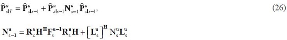
The fixed-interval smoothed estimates are instead given by working backwards from  with the following recursion:
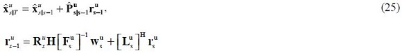
With ruT for s = T – 1, T – 2,...,1 and the associated variance-covariance matrices of the smoothed prediction error given by:
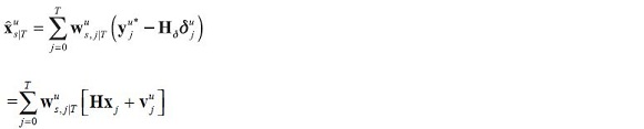
The one-step ahead predictions of the data are given by:

and the smoothed predictions follow a process:

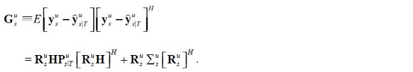
The variance-covariance matrix of the forecast error in the smoothed predictions of the fitted data at time s conditional on the information set u,  is given by:
The forecasts and fitted values of our model, which are identical to the expectations of agents, are given as:

Equation (28) is possibly the most important in the paper, linking the estimates from the algorithm using the data to the expectations of agents. It can be thought of as an assumption, as it would not hold if information sets of agents and the policy modellor were not symmetric. The Kalman filter algorithm also gives us other useful statistics which we can use in analyzing and presenting the forecast, as we shall do later on.
V. PHILOSOPHIES FOR FINDING PARAMETER VALUES FOR THE DATA MEASUREMENT EQUATION
To make this idea operational, we need to describe the schemes to find values for the matrices  and
and  that describe the data measurement system.
A. TENDER LOVING CARE
Priors for each of the elements of these matrices could be justified and imposed on a case by case basis, and the rest estimated. Provided the estimations are identified, a large degree of generality could be allowed for here. The model could be estimated in separate parts (ignoring some of the interrelations) or it could be estimated together,or in blocks. In any case, an appropriate estimation method, probably Bayesian, which balances prior information against data information, could be applied to the problem. As the priors are not automatic, and both the state-space and the data set could be very large, this could be costly to carry out and possibly even to maintain. But this might well be the most accurate method for building the data uncertainty part of the model, and may be what is needed if the demands of policy are such that the forecasts have to be consistent with all monitored indicators.
B. PURPOSE-BUILT DATA SET
The most common method used to construct the data set for a forecasting model is by finding one data series to match each important state variable. However, there will be some series —for example, the Lagrange multipliers or the flexible price variables— for which no good data series is available at all. They could be left to be solved within the model.
For those variables for which there is a series in the data set, the choice of H is straightforward: where the model concept has a series to match a state variable, the row and column H would serve as an identity matrix. For example, if the national accounts GDP data corresponds to the value-added output in the model and GDP is the nth data series and value-added output the mth state variable, H will have a 1 in entry (m, n) and zero elsewhere in the mth row and the nth column. Even if it can be assumed that that data series might on average rise and fall alongside the model concept, there is less reason to argue that it will be unbiased or without some noise. On these grounds, some systematic bias,  , and some data measurement error,
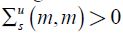 , might be allowed to interfere in these relations.
Where the model concept has no data, the consistent and transparent solution would be to eliminate that row in H and let the model solve for these series, by combining the available data with knowledge of model structure and parameter estimates.
This method is less costly, as data series are chosen essentially based on only what state variables are important in the model. But the forecasts may be much worse than an approach that also considers what useful data is available in designing the match. The purpose-built data set ignores the useful technology that is in this paper for bringing in other useful data.
C. EXTENDING THE MODEL TO FIT IN DATA
Yet, there may be variables which are not needed in the core solution of the model, but for which there is useful data. It can be very valuable to extend the model to include data from these variables for two reasons. First, if that data is informative it should directly improve the forecast. Second, if that data is what agents and policymakers use, the model will need to incorporate that data if it is to predict their behaviour well. One example is that of money aggregates which on occasion provide very useful and timely information for monetary policy, but which do not play a critical part in the solution of many DSGE models. Another example is when there is only annual data available for a quarterly model.
It is assumed that there are NM of these variables, called ms and that can be written as a static function of the variables in the model:

with each εm,s, is other and εs uncorrelated  non-singular. The key assumption here is that the solution for these variables can take place in a second stage after the main model has been solved. For example, assume that annual data is only available on a flow series, such as GDP:

where yas, is the data on the annual series and Zq,s-i is the unobserved (seasonally adjusted) quarterly state, and where both the annual and quarterly series are expressed in terms of log deviations of steady state. This could be introduced into the model in the form of equation (29).
Let us assume that these variables are related to the data according to the equation:
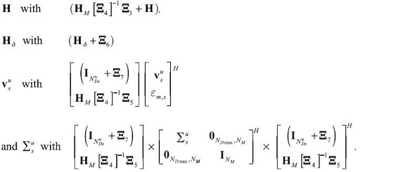
Therefore, this extension of the model can be built in by adapting the measurement equation according to:
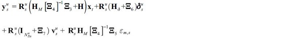
The rest of the results of the paper would follow if the following replacements were made in the measurement equation:
If the form (29) is not justified, then the original system would have to be enlarged to incorporate this information.
D. DATA INTENSIVE METHODS
At the other extreme, very many data series, many more than there are states, could be included, as in Boivin and Giannoni (2006). With very many data series, it will be infeasible to separately impose priors on the elements of the matrices linking each data series to each unobserved state variables. What might be possible is to group the data series in terms of which state variable they contain some useful information for, with the groups not necessarily being exclusive. There would be, at most, N groups of data.
One possible identifying assumption is that the common information that this group contains is proportional to the state variable that indexes that group. Standard dynamic factor analysis methods can be used to estimate and forecast each state variable, with the added twist here that the unobserved behaviour of the state variables is restricted to be consistent with the economic model.
E. SOME GENERAL PRINCIPLES TO CHOOSE THE DATA MEASUREMENT UNCERTAINTY
A more difficult decision is the choice of . Imposing case-by-case priors and estimating will almost certainly be infeasible, and also unidentifiable. It would be better to impose some structure to reduce the degrees of freedom. One solution could be to assume some process for the variance to increase slowly over the sample, starting from time 0 up until the end of the forecast, but with that rate of increase slowing down. The idea is to then estimate, or calibrate, that process, taking each series at a time —or much more ambitiously— to estimate the series of the matrices as a whole. But, there may be some uneven heteroskedasticity around the current period because of the calendar of national accounts release. This could be dealt with by splitting the data set into three periods and by putting in slope dummies into the variance process to adjust for the regime shift.
• The first period goes from time 0 to time T1, and takes us up to two quarters before the current quarter for which national accounts data is available.
• The second period is from time T1 to time T2 which is two quarters after the current quarter. Within this year, centered on the current time, judgement plays a major role.
• The final period is from time T2 up until the end of the forecast at time T.
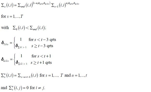
For each data series, the  data measurement variances across both time and information sets are summarised by five parameters: a starting value
  , a final value
  , a rate of improvement α, and two slope dummies to separate out the window surrounding the current time,
  and
and  . If a real time data base were available, that could be used to set estimates of the scale of data uncertainty at a particular lag, for example at t – 3, and through that same route to estimate
  . These kinds of estimates should help pin down values of the parameters here.
VI. USEFUL OUTPUTS FROM THE FORECASTING SYSTEM
A policy forecast is judged not just on its predictability, but also on how well it tells stories. Indeed, often the job of the policy forecaster is to explain what went wrong! In order to do this, it is important to be able to decompose the forecast into two dimensions: first, in terms of the data and second, in terms of the economic and data measurement shocks. The contributions on either dimension are myriad, and so it is also important to think of interesting ways of summarising this information. Finally, it would be useful to have a metric for assessing the information worth of bits of data or whole series.
A. DATA DECOMPOSITIONS
Consider the multiplier matrices 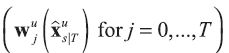 , which when multiplied by the selector matrix
  determine how much each piece of information (data plus adjustments) from the mythical full data set at time s based on the information set affects the smoothed estimate at time s. These multipliers are defined by the relationship:

Define the matrices 
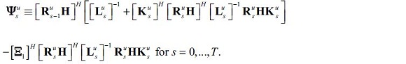
Then, the multiplier matrices are calculated in part backwards and in part forwards from time s. The recursion formulas from Koopman and Harvey (2003) are:


The contributions of each piece of data to these estimates are then simply that piece of data multiplied by its multiplier, only that here they are also indexed by the information sets through u.
Publishing forecasts is about communications as much as anything else. But, if the central bank wants to communicate with the public, it should always refer to data that is publicly and objectively available1. For that reason, it is also important to present the contributions of data to the smoothed estimates of the data series themselves. These are given by:

A popular maxim in policy forecasting is that it is the source of the shock that matters, meaning that the explanations of the forecast depend very much on what shocks are believed driving the forecast. It would therefore be useful to know how we determine these shocks; in terms of which bits of data tell us that there is a demand versus a supply side shock, for example. The economic shocks are given as
the last members of the state vector, and so equation 6.1 can be used to generate this interesting decomposition.
1. Summarizing the Information Given by the Data Decompositions
The decompositions in this section provide a myriad of information. It is usually convenient to summarize that information along some relevant dimension. There are many interesting possibilities; but three standard aggregations spring to mind:
1) The contribution of each individual data series in a given set is given by adding up the contributions of observations on each series over time.
2) The impact of the news in each data series on each forecasted variable can be calculated by subtracting the contribution of each data series as it was in the previous information set from the contribution of that series as it is in the current data set.
3) The data set into the part that reflects off -model judgement and the rest.The role of judgements is then the sum of the contributions of those pieces of data which are designated to be judgement.
4) These calculations can only be in terms of the contribution exclusive to key variables, for example inflation and GDP, and then only over the more interesting periods, such as the forecast.
2. The Information Contribution of Each Piece of Data to the Forecast
The expected contributions of particular pieces of data to the forecasted variable were derived previously in this section. It is interesting to complement that with some measure of how much useful information each data series brings to the forecast, which can be thought of as a forecast error variance decomposition in terms of the data series.
Tinsley, Spindt, and Friar (1980) and later Coenen, Levin, and Wieland (2004) describe how the information contribution of a piece of data to a forecast is related to the reduction in uncertainty that using that data brings to the forecast. The expected uncertainty in two sets of variables x and y is defined as:

where f (y,x) is their joint density. Consistently the uncertainty in just y is:

where f (y) is the marginal density of y, and the conditional uncertainty of y given x is:

where f (y | x) is the conditional density of y given x. The mutual information content of x and y is then defined by the reduction in expected uncertainty when x is used to predict y:

and is always positive definite. If y and x are jointly normally distributed, Tinsley, Spindt, and Friar (1980) show that the mutual information content is then:
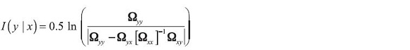
where Ωz1z2 is the covariance matrix between two vectors z1 and z2S. If x is partioned into two sets of information, the extra gain in using x1 alongside x2 over just using x1 is G(y | x1, x2) where:
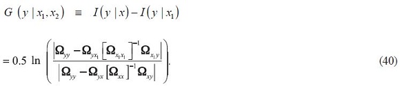
This is the percentage difference between the square root of the determinant of the conditional variance covariance matrix of y just using x1 and the square root of the determinant of the conditional variance covariance matrix using both x1 and x2. As such it seems to be a good measure of the marginal information content of x2 over and above x1. Note that it is not the same as mutual information content of y and x2, which is I (y | x2).
This measures the information value to estimating all the states in the forecast over the whole sample. But, what is more likely to be of interest is to assess the information content of a data series in terms of predicting just one state variable, and even then, over a particular time window. For example, the relevant question might be, how useful is a particular data series in predicting inflation over the two-year forecast horizon? An appropriate answer would then be given by the following statistic based on a scalar version of (40) above.
Proposition. The extra information content of the jth data series in predicting the ith variable on average over the two year forecast horizon could then be measured by:
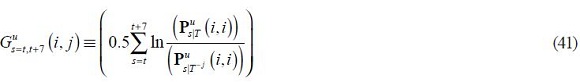
where the ith variable is of interest, t is the current time and the frequency is quarterly, and T-j indicates that all but the jth data series whose information content we want to measure to calculate the covariance of the states is being used.
B. EXTRACTING INFORMATION ON THE ECONOMIC CONTENT OF THE MODEL
It is also interesting to see to what extent the forecasted values are driven by economic shocks. The economic content of the model can also be presented as impulse responses or variance decompositions as in Gerali and Lippi (2003).
1. Economic Decompositions
The last state variables describe the exogenous economic shocks, also in terms of when they were first spotted.  refers to the vector of state estimates of those state variables at time s using information set u. The lower partition described in equation (15) and these smoothed state estimates to recover smoothed estimates of the white noise components of these shocks as:

Then the contribution of the ith shock to the smoothed estimate at time s on information set u is:

where Rεi is a ![]() matrix formed by taking an identity matrix and putting zeros in all but the ith diagonal element. The contribution to the smoothed fitted values of the data series will be:
matrix formed by taking an identity matrix and putting zeros in all but the ith diagonal element. The contribution to the smoothed fitted values of the data series will be:

.
Here, it should be remembered that the sum of the contributions across all shock will equal the smoothed estimate of the data series minus the mean bias terms 
2. Impulse Responses
To obtain the economic decomposition of the states, the decomposition is first written as:
where the  matrices
  , are given by
 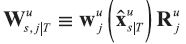 .
.
Substituting out for the true states gives:
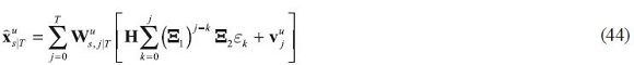
which decomposes the state estimate into the contribution of each economic shock and each data noise shock. Impulse responses to economic shocks or data errors can now be derived from expression (44).
Similarly, the smoothed estimates of the data and the policy interest rate can be decomposed into shocks with a view to obtaining the impulse responses to the fitted data values:

3. Variance Decompositions
The variance decomposition of a state estimate is the proportion of variance explained by the variance of each type of shock at each horizon. The unconditional variance of the state estimates is first derived as:
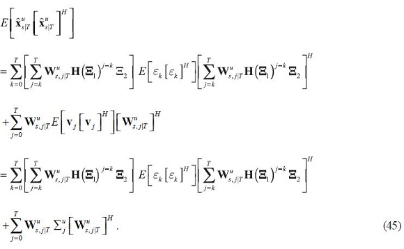
Given a suitable calibration about the variance-covariance matrix of economic shocks 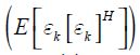 which could be an identity matrix, expression (45) permits the decomposition.
It would be useful to draw bands of uncertainty around the forecasts. The forecast error of the estimated state variable is:
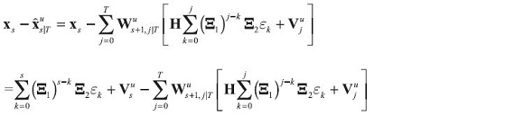
So, if by defining the matrices  such that:
then the forecast error covariance of the state estimates can be written as:
Similarly the covariance of the estimates of the fitted variables is:

with the covariance of the forecast error of fitted data in terms of shocks as:

It should be noted, however, that these expressions do not take account of estimation uncertainty. That would seem to be more obviously deficient in a set up where the data are formally separated from the model variables. In our opinion, then, these expressions should be superceded by a formal combined treatment of uncertainty and estimation, and by one which is designed for policy. Such a scheme is outlined in Sims (2002) and applied by Adolfson, Andersson, Lindé, Villani, and Vredin (2005).
VII. ALLOWING FOR REPORTING VARIABLES
One way to better exploit this wealth of information, is to introduce variables into the economic model which are there just for reporting. This is a very common practice in policy forecasting as round by round the way the forecast is presented changes depending on particular issues.
Formally, the reporting variables could follow the process:

where  is a vector of white noise residuals, allowing for the fact that reporting is not exact. Schorfheide, Sill, and Kryshko (2010) discuss the importance of allowing for these non-modelled variables and suggest how such auxiliary equations can be estimated. Here, more simply, the variance of these residuals is assumed to be given.
In keeping with the spirit of what a reporting variable is it is also assumed that these residuals are independent of the shocks and data noise terms in the rest of the model. Otherwise these variables would have to be incorporated into the model. The smoothed estimates of the reporting variables are:

Then, the forecast of these variables can be decomposed into the contributions of economic shocks with:

from equation (43).
The impulse responses are:
and the variance decomposition follows:

The variance-covariance matrix of forecast errors is:

VIII. THE STATE IDENTIFICATION PROBLEM
An identification problem arises when the values of parameters cannot be separately estimated given the combination of a theoretical model and a data set. This type of identification problems bedevils the estimation of DSGE models: see Canova and Sala (2006), Fukac and Pagan (2006) and Guerron-Quintana (2007) and recently Koop, Pesaran, and Smith (2011). Here, it is assumed that the parameter values are known; and so, that particular problem has been set aside. However, it is still very possible that there is an identification problem in the estimates of state variables: the data and model together might fail to separately identify some states. Indeed, as the solution for states is a first step in the recursions used to estimate parameters; for example, as in maximum likelihood estimation, state identification could be seen a necessary condition for parameter identification. These problems are not generic to the proposal in this paper, but this procedure will certainly bring these problems to
the fore. Therefore, it is worthwhile to spend some time discussing the problem of state identification.
Weak identification can be expected to especially affect our estimates of the economic shocks. Remember that economic shocks have no direct data counterpart to which their value can be tied down. Then, it becomes more likely that the forecast of a variable —even on which good data is available— is based on very unreliable estimates of what shocks cause those movements.
There are many different ways in which these problems can show themselves, if one digs deep enough.
One classic symptom would be if the estimates of two shocks that affect one variable for which there is a data counterpart were estimated to have large, but offsetting, contributions. Another would be if the estimate of a shock failed to update from its initial prior value. A different way of looking at this problem is to note that the data series are not separately informative about state estimates, and are in this sense multicollinear. This then points to yet another symptom: one which would be where the estimates of particular states were too sensitive to changes in the data set, as explained in Watson (1983).
One subcategory of this shock identification problem is when data measurement errors cannot be separately estimated from economic shocks. This could reveal itself when the estimate of a data measurement error were negatively correlated with the economic shock. Remember that the covariances between data measurement and economic shocks are assumed to be zero. Relaxing that assumption would be more realistic but would also expose us to more identification errors of this type.
It is difficult to offer general solutions to state identification problems. It is important to remember that a failure of identification has to do with the flawed combination of model and data —and with neither individually—.
Thus, there may be some shocks that can be identified with some data but not with others. And, there may be some shocks which are not identifiable by any data that are available! The solution to identification may lie either in changing the model; or, in looking for new data; and will probably involve some compromises in either or both directions. Solutions would seem to be case by case.
But, it is possible to formulate general tests to detect identification problems. Burmeister and Wall (1982) offer one test for the identification problems for parameter estimates in state space models. Their suggestion is to keep an eye out for very large correlations among parameter estimates. Analogously, here high correlations among the estimates of the economic shocks would reveal poor identification.
The variance-covariance matrix of the impact of the economic shocks (which are included in the state vector) is given in equation (45). Then, the following test can be constructed.
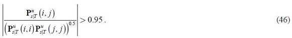
Proposition. Given an information set u, the estimate of the economic shock impacts i and j at time s are not likely to be well identified separately if:
The identification problem can also be assessed from the point of view of whether adding a particular series to a given data set brings in more information in identifying a group of variables, using test (41).
IX. SOME APPLICATIONS
In this section some experiments from applying this approach to a quarterly DSGE model for Colombia are reported. The model (PATACON) is described in Gómez, Mahadeva, Sarmiento, and Rodríguez (2011). It is an open economy model which has been calibrated to fit Colombian data for the period 2003-2006. The database, of a quarterly frequency, runs from 1994Q1 to 2006Q4, is described in Mahadeva and Parra (2008).
A. A COMPLETE FORECAST
To begin with, the first aim is to show that this model, and its database, is at least capable of generating a decent forecast. One can, in principle, generate a forecast with very little data, but that forecast could be quite poor. Adding more data can in principle improve that forecast. The Graphs 2 and 3 show the forecasts of the model for quarterly real value-added income (nominal GDP divided by the CPI) growth. Twelve series are included in the data base up until period 40 (10 years of data), and it is assumed that they are all perfectly measured. In this experiment, the model allows for 12 structural shocks all of which seem to be reasonably well identified.
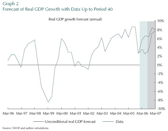
The first Graph presents the forecast with no other data beyond the 40 quarters´ cutoff point. The forecast in the second Graph is based on an extra two quarters of inflation, interest rate, and real exchange rate data.
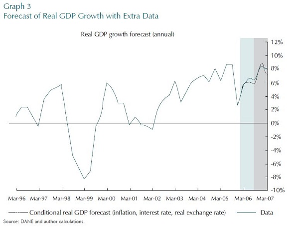
Comparing the two forecasts makes the simple point that this model is capable of making a decent forecast, but only if the information on recent data is included. This is true even if that information is from other series, given that the theoretical part of the model is able to interpret the linkages between these series.
B. EXPERIMENT TO SHOW THE IMPORTANCE OF IMPERFECTLY MEASURED AWKWARD DATA
This next set of experiments is about the advantage of allowing for measurement error in unbalanced data. The first in this next set of experiments uses data on consumption and inflation only until period 47 and no more, and assumes that both series are well measured. The results are in Graph 4. Then, three extra quarters of data on CPI inflation are introduced, while still assuming that both those series are well measured. This is a very similar exercise to that of the previous section. Comparing Graph 4 with Graph 5, it seems that the extra data on CPI ensures that the boom in consumption in between periods 47-52 picked up.
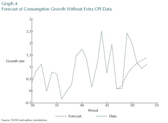
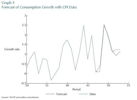
However, we should be careful about leaping to the conclusion that more data always improves a forecast. All that has been shown is that the extra data on prices helps the forecast track consumption better. If those extra two data points in the CPI were badly measured, then what we have produced is an even worse forecast. This is a very real possibility in Colombia because the statistical authority only updates its aggregate CPI weights once every five years, and then even near term forecasts are subject to measurement error.
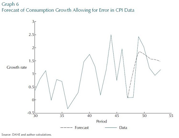
To expand further on this point, the next experiment compares the previous two forecasts with one in which we allow for data mismeasurement in the extra three CPI data points, in Graph 6. This forecast is now a compromise between the two others; and, perhaps, reflects a better balance between not ignoring important data and not chasing it too closely.
C. EXPERIMENTS TO SHOW THE IMPORTANCE OF OFF-MODEL FORECASTS
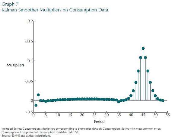
The next set of Graphs illustrates the use of the data decompositions. In what follows, there are only two economic shocks, a demand and a supply shock, and it is assumed that the supply shock dominates. In the first experiment there is only noisy data on consumption. The task is to predict all variables in the model, including true consumption itself. Graph 7 shows the multipliers of consumption data in predicting true consumption in period 45 in this experiment. Notice that the distribution is symmetric about the current period. Given that there are measurement errors, surrounding data helps to estimate the unobserved state at the current period: only that here, that pattern reflects in part the dynamics of the DSGE model.
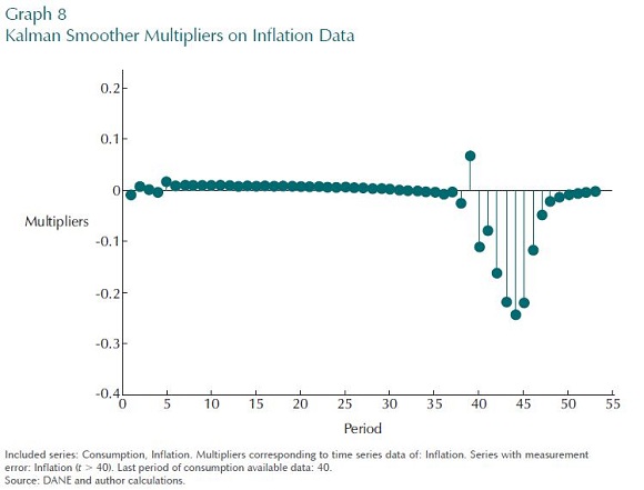
The next experiment looks into exactly how the information from off-model forecast of inflation in the short term helps in predicting consumption now. The experiment assumes perfectly measured data on consumption and inflation only until period 40, and then inflation data only for the next two years. These extra two years of inflation data are assumed to have measurement error, just as if they were forecasts from a separate inflation model.
The multipliers on estimating consumption in period 45, shown in Graph 8, describe how inflation data —even a year ahead— plays some part in helping us understand what is happening to consumption in the absence of timely consumption data. The multipliers are negative because higher prices imply a lower level of consumption, conditional on the supply shock being important. Shown this figure, a policymaker would understand how his/her off-model inflation forecast would be consistent with his/her forecast for consumption, and so ultimately with GDP.
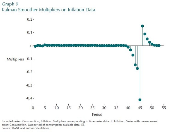
This can be compared to a forecast with data on both consumption and inflation up until period 53. Consumption is imperfectly measured, but the inflation data is assumed to be without error. Graph 9 plots the multipliers on inflation data in predicting consumption at period 45. It is interesting to see that the multipliers on future inflation data are now positive in predicting current consumption. This has to
do with the economic dynamics of the model. Given that the supply shock is important, higher prices now mean lower consumption level now, and so higher prices in the future mean lower consumption expected in the future. Intertemporal consumption dictates that lower expected consumption in the future would raise consumption now and so the multiplier on future inflation data is positive.
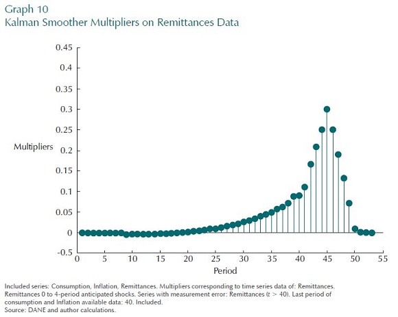
Data about the future in the form of forecasts from external sources can be useful but is uncertain. To bring this out, the next experiment examines the role of imperfectly credible announcements of future data outturns. In this experiment, the forecaster is assumed to be in period 40 and trying to forecast consumption a year ahead. Consumption and inflation data only up until period 40 are available and both those series are perfectly measured. Now, information is provided to agents and forecaster alike on what remittances are going to be for the next two years (from periods 41 to 49). Those announcements are not perfectly credible though; there is measurement error. The multipliers reveal how that future imperfect information on an important exogenous variable matters for the forecast of consumption in period 45. This could also be presented by picking out the contribution to consumption growth in period 45 of the remittance data. In more sophisticated experiments, this technology can be used to explain the importance of financial market data on the expected future values of asset prices on forecasts of macroeconomic variables.
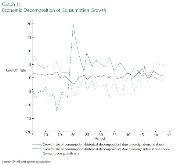
D. EXPERIMENT TO REVEAL THE IDENTIFICATION PROBLEM
The Graph 11 illustrates the identification problems that we discussed in section VIII. The figure shows the contribution of two main shocks to consumption growth when we do not allow for measurement error in the CPI, and when it is assumed that there are only two economic shocks. The model has picked up what it identifies as being a very large offsetting contribution of the two shocks. It does not seem likely that these really have had offsetting effects on consumption, but rather that the model and data cannot separately identify the contribution of each, only their linear combination.
X. CONCLUSIONS
The data that is informative for making monetary policy decisions comes in many shapes and sizes and is uncertain. In this paper, we propose one possible way of putting that awkward, but still useful, data set to work in forecasting from a linear dynamic forward-looking model.
There are some important practical advantages to this approach. First, it allows theoretical models access to the rich set of real world data that is actually in use. The method also stimulates different ways of presenting and explaining the forecasting. For example, we can present a forecast in terms of what data explains the decisions over key variables, and not just what set of shocks causes that forecast. The difference is that as the data is observed the forecast becomes more transparent. We also show how this method can cope with less than perfectly credible announcements of future information, such as that contained in financial market data. Last, but not least, this method has the advantage of separating the data preparation process from the model formulation and solution process. This would better suit how central banks carry out their policy forecasts in practice, given that these two activities are quite specialized.
That said, although we consider this approach to be a step forward, there still remain some important aspects of the policy forecasting problem which have not been taken into account.
First, we do not deal with the possibility of inevitable misspecification, a recent preoccupation of the DSGE literature (Negro and Schorfheide, 2009); even though, as Maih (2010) shows, the benefits of conditioning depend crucially on misspecification. An important source of misspecification and forecast error in DSGE models is down to drift in economic relations, which are assumed to be fixed in the steady state of these models. For example, it is often observed that the imports to GDP and exports to GDP ratios rise persistently with greater openness. Our data uncertainty method is not designed to deal with such trending economic shocks.
Second, we do not discuss how the parameters of the economic model are estimated or calibrated. We discuss alternative procedures for estimating the measurement system that links the data to the unobserved economic model, but we do not do that in much depth. As such, we do not allow for parameter estimation effects in this decomposition of the contributions of different data series. Neither have we yet tackled the problem of estimating the whole distribution of these impulse responses and decompositions of the forecasts, and not just the mode value, as this would need to take account of parameter estimation uncertainty. We do provide some expressions for the asymptotic conditional uncertainty of the forecast; but without formal treatment of estimation uncertainty, we cannot claim that this is a serious presentation of the forecast distribution.
We do not allow for second-order approximations of the form popularised by Schmitt-Grohé and Uribe (2004). Nor do we allow for asymmetric risks in the forecast which has become common central bank practice following Britton, Fisher, and Whitley (1998).
Finally, as the set up here is based on a linear model, or more precisely a linearised version of a nonlinear model, this strategy does not apply to nonlinear solution methods, such as that presented in Laxton and Juillard (1996) and Pichler (2008). It is our hope that we, and others, will be able to apply some common solutions to these problems within our apparatus.
COMENTARIOS
1 See a parallel literature on assessing optimal policies in linear rational expectations models under data uncertainty following papers by Gerali and Lippi (2003), Pearlman (1986), Svensson and Woodford (2003) and Svensson and Woodford (2004).
2 Data and economic shocks will also be correlated in the complicated case that information is
not symmetric between agents and the modellor.
REFERENCES
1. M.; Lindé, J.; Villani, M.; Vredin, A. "Modern Forecasting Models in Action: Improving Macroeconomic Analyses at Central Banks", Working Paper Series, num. 188, Sveriges Riksbank (Central Bank of Sweden), 2005. [ Links ]
2. Andersson, M. K.; Palmqvist, S.; Waggoner, D. F. "Density-Conditional Forecasts in Dynamic Multivariate Models", Working Paper, num. 247, Sveriges Riksbank, 2010. [ Links ]
3. Benes;, J.; Binning, A.; Lees, K. "Incorporating Judgement with DSGE Models", Reserve Bank of New Zealand, Discussion Paper Series, num. DP2008/10, Reserve Bank of New Zealand, 2008. [ Links ]
4. Boivin, J.; Giannoni, M. "DSGE Models in a Data-Rich Environment", Working Paper, num. T0332, NBER, 2006. [ Links ]
5. Boragan Aruoba, S. "Data Uncertainty in General Equilibrium", Computing in Economics and Finance, num. 131, Society for Computational Economics, 2004. [ Links ]
6. Britton, E.; Fisher, P.; Whitley, J. "The Inflation Report Projections: Understanding the Fanchart", Quarterly Bulletin, num. 1, Bank of England, 1998. [ Links ]
7. Burmeister, E.; Wall, K. "Kalman Filtering Estimation of Unobserved Rational Expectations with An Application to the German Hyperinflation", Journal of Econometrics, vol. 20, num. 2, pp. 255-284, 1982. [ Links ]
8. Canova, F.; Sala, L. "Back to Square One: Identification Issues in DSGE Models", Working Paper Series, num. 583, European Central Bank, 2006. [ Links ]
9. Coenen, G.; Levin, A.; Wieland, V. "Data Uncertainty and the Role of Money as an Information Variable for Monetary Policy", European Economic Review, vol. 49, num. 4, pp. 975-1006, 2004. [ Links ]
10. Durbin, J.; Koopman, S. Time Series Analysis by State Space Methods (vol. 24), Oxford Statistical Series, Oxford University Press, 2001. [ Links ]
11. Fukac, M.; Pagan, A. "Issues in Adopting DSGE Models for Use in the Policy Process", Working Papers, num. 2006/6, Czech National Bank, Research Department, 2006. [ Links ]
12. Gerali, A.; Lippi, F. "Optimal Control and Filtering in Forward-Looking Economies", Working Paper, num. 3706, Centre of Economic Policy Research, 2003. [ Links ]
13. Gómez, A. G.; Mahadeva, L.; Sarmiento, J. D. P.; Rodríguez, D. G. "Policy Analysis Tool Applied to Colombian Needs: PATACON Model Description", Borradores de Economía, núm.
008698, Banco de la República, 2011. [ Links ]
14. Guerron-Quintana, P. A. "What You Match Does Matter: The Effects of Data on DSGE Model Estimation", Working Paper, North Carolina State University, 2007. [ Links ]
15. Harvey, A. Forecasting, Structural Time Series Models and the Kalman Filter, Cambridge, Cambridge University Press, 1991. [ Links ]
16. Kalchbrenner, J. H.; Tinsley, P. A.; Berry, J.; Garrett, B. "On Filtering Auxiliary Information in Short-Run Monetary Policy", Carnegie-Rochester Conference Series on Public Policy, vol.
7, num. 1, pp. 39-84, 1977. [ Links ]
17. Klein, P. "Using the Generalized Schur Form to Solve a Multivariate Linear Rational Expectations Model", Journal of Economic Dynamics and Control, vol. 24, num. 10, pp. 1405-1423, 2000 [ Links ]
18. Koop, G.; Pesaran, M. H.; Smith, R."On Identification of Bayesian DSGE Models", Working Papers, num. 1108, University of Strathclyde Business School, Department of Economics, 2011. [ Links ]
19. Koopman, S.; Harvey, A. "Computing Observation Weights for Signal Extraction and Filtering", Journal of Economic Dynamics and Control, vol. 27, num. 7, pp. 1317-1333, 2003. [ Links ]
20. E. "Anticipated Alternative Policy Rate Paths in Policy Simulations", International Journal of Central Banking, vol. 7, num. 3, pp. 1-35, 2011. [ Links ]
21. Laxton, D.; Juillard, M. "A Robust and Efficient Method for Solving Nonlinear Rational Expectations Models", IMF Working Papers, num. 96/106, International Monetary Fund, 1996. [ Links ]
22. Leeper, E. M.; Zha, T. "Modest Policy Interventions", Journal of Monetary Economics, vol. 50, num. 8, pp. 1673-1700, 2003. [ Links ]
23. Lettau, M.; Ludvigson, S. "Understanding Trend and Cycle in Asset Values: Reevaluating the Wealth Effect on Consumption", American Economic Review, vol. 94, num. 1, pp. 276-299, 2004. [ Links ]
24. Mahadeva, L.; Parra, J. C. "Testing a DSGE Model and its Partner Database", Borradores de Economía, num. 004507, Banco de la República, 2008. [ Links ]
25. Maih, J. "Conditional forecasts in DSGE models", Working Paper, num. 2010/07, Norges Bank, 2010. [ Links ]
26. Monti, F. "Combining Judgment and Models", Journal of Money, Credit and Banking, vol. 42, num. 8, pp. 1641-1662, 2010. [ Links ]
27. Negro, M. D.; Schorfheide, F. "Monetary Policy Analysis with Potentially Misspecified Models", American Economic Review, vol. 99, num. 4, pp. 1415-1450, 2009. [ Links ]
28. Orphanides, A. "Monetary Policy Rules Based on Real-Time Data", American Economic Review, vol. 91, num. 4, pp. 964-984, 2001. [ Links ]
29. Pearlman, J. "Diverse Information and Rational Expectations Models", Journal of Economic Dynamics and Control, vol. 10, num. 1-2, pp. 333-338, 1986. [ Links ]
30. Pichler, P. "Forecasting with DSGE Models: The Role of Nonlinearities", The B.E. Journal of Macroeconomics, vol. 8, num. 1, p. 20, 2008. [ Links ]
31. Robertson, J. C.; Tallman, E. W.; Whiteman, C. H. "Forecasting Using Relative Entropy", Journal of Money, Credit and Banking, vol. 37, num. 3, pp. 383-401, 2005. [ Links ]
32. Schmitt-Grohé, S.; Uribe, M. "Solving Dynamic General Equilibrium Models Using a Second- Order Approximation to the Policy Function", Journal of Economic Dynamics and Control, vol. 28, num. 4, pp. 755-775, 2004. [ Links ]
33. Schmitt-Grohé, S.; Uribe, M. "What's News in Business Cycles", Working Paper, num. 14215, NBER, 2008. [ Links ]
34. Schorfheide, F. "Estimation and Evaluation of DSGE Models: Progress and Challenges", Working Papers, num. 16781, National Bureau of Economic Research, Inc., 2011. [ Links ]
35. Schorfheide, F.; Sill, K.; Kryshko, M. "DSGE Model-Based Forecasting of Non-Modelled Variables", International Journal of Forecasting, vol. 26, num. 2, pp. 348-373, 2010. [ Links ]
36. Sims, C. A. "Solving Linear Rational Expectations Models", Computational Economics, vol. 20, num. 1-2, pp. 1-20, 2002. [ Links ]
37. Svensson, L. E.; Woodford, M. "Indicator Variables for Optimal Policy", Journal of Monetary Economics, num. 50, pp. 691-720, 2003. [ Links ]
38. Svensson, L. E.; Woodford, M. "Indicator Variables for Optimal Policy under Asymmetric Information", Journal of Economic Dynamics and Control, vol. 28, pp. 661-690, 2004. [ Links ]
39. Tinsley, P.; Spindt, P.; Friar, M. "Indicator and Filter Attributes of Monetary Aggregates: A Nit-Picking Case for Disaggregation", Journal of Econometrics, vol. 14, num. 1, pp. 61-91, 1980. [ Links ]
40. Uhlig, H. "A Toolkit for Analyzing Nonlinear Dynamic Stochastic Models Easily", Discussion Paper, num. 9597, Tilburg University Center, 1995. [ Links ]
41. Watson, P. "Kalman Filtering as an Alternative to Ordinary Least Squares-Some Theoretical Considerations and Empirical Results", Empirical Economics, vol. 8, num. 2, pp. 71-85, 1983. [ Links ]
