


Services on Demand
Journal
Article
 English (pdf)
 Article in xml format
 Article references
 Send this article by e-mail
Indicators
-
 Cited by SciELO
 -
 Access statistics
Related links
-
 Cited by Google
 -
 Similars in
SciELO
Similars in
SciELO -
 Similars in Google
Share

 Permalink
Ensayos sobre POLÍTICA ECONÓMICA
Print version ISSN 0120-4483
Ens. polit. econ. vol.32 no.spe73 Bogotá Jan. 2014
Macroeconomic Stabilisation and Emergency Liquidity Assistance
Estabilización macroeconómica y asistencia de liquidez de emergencia
Marcelo Sáncheza
a European Central Bank, Frankfurt am Main, Germany
E-mail address: marcelo.sanchez@ecb.int
History of the article:Received June 19, 2013 Accepted October 25, 2013
ABSTRACT
We introduce imperfect monetary policy transparency and strategic wage setting into a macro model where the central bank provides lender of last resort (LOLR) services to banks on top of its standard stabilisation policy. We study how, in the presence of adverse exogenous financial developments, macroeoconomic and financial instability can be dampened by adjustments in policy institutions and economic structure. In a context of costly LOLR transactions and no moral hazard, the central bank has an incentive to save only large banks. Central bank opaqueness can help improve macroeconomic and financial stability by making wages closer to their competitive levels. Some results depend on initial conditions concerning monetary institutions; for instance, monetary strictness and wage bargaining centralisation help discipline wages and thus are stability-enhancing when central bank policies are initially seen as rather strict and transparent. Some consideration is given to the roles of trade openness and moral hazard behaviour on the part of banks.
Keywords: Macroeconomic stabilisation, Lender of last resort, Banking crises, Monetary accommodation, Central bank transparency, Wage bargaining.
Jel Classification: E50, E52, E58, G21, G28, J51.
RESUMEN
Introducimos imperfecciones en la transparencia de la política monetaria y fijación estratégica de salarios dentro de un modelo macro donde el banco central provee servicios de prestamista de última instancia (PUI) a bancos comerciales además de la habitual política de estabilización. Estudiamos cómo, en presencia de eventos financieros adversos de carácter exógeno, la inestabilidad macroeoconómica y financiera puede ser amortiguada a través de ajustes en las instituciones políticas y la estructura económica. En un contexto de transacciones de PUI costosas y ausencia de riesgo moral, el banco central tiene un incentivo a rescatar sólo bancos grandes. La opacidad del banco central puede ayudar a mejorar la estabilidad macroeoconómica y financiera al inducir los salarios a aproximarse a su novel competitivo. Algunos resultados dependen de las condiciones iniciales relativas a las instituciones monetarias; por ejemplo, la restricción monetaria y la centralización en las negociaciones salariales ayudan a disciplinar los salarios y así a estabilizar la economía cuando la política monetaria es inicialmente percibida como bastante estricta y transparente. Damos alguna consideración a los roles de la apertura comercial y al comportamiento de riesgo moral por parte de los bancos.
Palabras clave: La estabilización macroeconómica, Prestamista de última instancia, Las crisis bancarias, Acomodación monetaria, La transparencia del banco central, La negociación salarial.
Clasificación JEL: E50, E52, E58, G21, G28, J51.
1. Introduction
In numerous countries the main goal of monetary policy is to maintain price stability. To do so, the central bank (CB) follows a policy rule enjoying a substantial degree of independence. Suitably designed, monetary policy rules may deliver price stability as well as maintain output close to its potential. The ongoing worldwide financial crisis has made clear that, beyond price stability, financial stability (comprising the provision of CB liquidity and the use of prudential rules) is and remains an essential objective. In recent years, there has been a sizeable increase in the provision of lender of last resort (LOLR) services to individual commercial banks, whereby CBs stand ready to inject high-powered money into the banking system whenever a bank is solvent but suffers from temporary liquidity problems.1 LOLR services to individual commercial banks have been a common practice, although in theory failures of banks could be prevented by implementing appropriate systems of bank regulation and supervision or private safety nets. These instruments are thus deemed insufficient to prevent CBs from intervening in the banking sector.
Despite the relevance of financial stability considerations, the economics profession does not offer a workhorse model for how macroprudential actions interact with the more traditional inflation-fighting role of monetary policy. It has been emphasised that, in the present context, multiple objectives require multiple instruments (Blanchard et al., 2012). But a better understanding is needed of issues such as what instruments should monetary and other authorities use to achieve these macroprudential goals, how large are the relevant trade-offs between macroeconomic performance and financial stability, and how economic uncertainty affects the conduct of CB policies.2
It has been argued that the CB should provide liquidity to the market and should not lend to individual banks, which would be able to borrow in the interbank market if they are considered to be solvent (Goodfriend and King, 1988). This view, however, assumes that interbank markets work perfectly and that the market is as well or better informed than the CB about the relative solvency of a bank short of liquidity. Moreover, LOLR transactions could obey to a macro rather than a micro motivation. Four valuable formal approaches have deviated from such view and contributed to understanding why CBs provide LOLR services:
-
First, some studies shed light on the question of why commercial banks might be reluctant to make use of LOLR services in connection with a coordination failure (Rochet and Vives, 2004). A coordination problem may arise when there is any large-scale need to redirect reserves, but there is no incentive for any individual commercial counterparty to sort out the problem by assuming the credit risk and undertaking the transaction costs involved. This occurred, for example, when the operation of many markets were severely disrupted as the Bank of New York computer malfunctioned in 1985 and in the events of September 11 (2001), when the Federal Reserve System hugely expanded its discount window lending to many individual banks (McAndrews and Potter, 2002).
-
Second, some authors focus on the micro-aspects of CB intervention in dealing with market failure. Using the framework of Diamond and Dybvig (1983), Freixas et al. (2004) analyse the moral hazard problem caused by bank managers' incentive to choose an inefficient technology that gives them some private benefit.3 In this asymmetric information context, liquidity shocks affecting banks might be undistinguishable from solvency shocks.4 Bianchi et al. (2012) model the interaction between credit frictions, financial innovation, and learning.5 In the decentralised equilibrium each household fails to internalise the effect of its borrowing decisions on asset prices, leading to excessive debt accumulation and too frequent crises. When the CB has better information than banks about the economic outlook, macroprudential policy would be justified since it can help offset the pecuniary externality generated by the collateral constraint.
-
Third, Goodhart and Huang (2005) assess the role of both contagious risks and moral hazard at the macro-level. If an illiquid, but solvent, bank is forced into closure, it is more likely that this will have significant adverse implications for the financial system as a whole the bigger that bank is. Thus, Goodhart and Huang's (2005) model in a static setting suggests that the CB would only rescue banks that are "too big to fail".6 The authors find that this result is broadly robust to a dynamic extension, in which setting contagious considerations dominate the role of moral hazard.
-
Fourth, Berlemann and Zeidler (2009) propose a model where the primary motive for providing LOLR transactions is macro rather than micro. The authors argue that, following the closure of commercial banks, fractional reserve banking systems are prone to liquidity crises whenever the public changes its preferences towards holding more high-powered money. In such a setting, LOLR transactions can contribute to lowering uncertainty about the money multiplier, and thus dampening variability in both inflation and output. Given the costs incurred in unsuccessful LOLR transactions, CBs have an incentive to save only the large banks, while the small banks are closed. A benevolent CB will thus accept greater macroeconomic variability when facing such LOLR costs.
The present paper examines the role of LOLR provision for macroeconomic stabilisation. LOLR provision, by adjusting banks' access to liquidity, can be combined with standard monetary policy to rebalance macroeconomic and financial stability. The main object is to investigate how the trade-off between financial instability and macroeconomic variability (as created -say- by financial shocks) can be improved by dampening fluctuations in inflation and output via adjustments in monetary institutions and the economic structure. Institutions (as given by the monetary policy setup, wage bargaining and the non-cooperative game involved between the CB and wage setters) affect the ability of policymakers to successfully undertake LOLR actions,7 as does the economic structure (as captured by the link between trade openness and the responsiveness of aggregate supply).
We start from a setup where the CB provides LOLR services to banks on top of its standard stabilisation policy, in the context of an endogenous determination of output distortions (operating via the labour market). Concerning the representation of the banking sector, we follow Goodhart and Huang (2005), who -in the presence of bank closures- assume that the public may move out of failing banks' deposits into cash, thereby reducing the money multiplier. Heightened financial strain raises both financial instability (directly) and macroeconomic variability (via bank closures and their implications for fluctuations in the money multiplier).8 LOLR transactions are aimed at mitigating part of the rise in overall instability. Moreover, we introduce imperfect monetary policy transparency and an explicit consideration of wage setters' preferences. This draws on Spyromitros and Zimmer (2009) and Sánchez (2011 and 2013), who study games between the CB and trade unions where the CB may be ambiguous about the policy weight of inflation relative to output.9 As a result, an endogenous output distortion arises from deviations of the wage rate from its competitive level, which are influenced by a number of institutional and structural factors. In this context, we are able to assess how monetary policy (in terms of the degrees of CB transparency and CB accommodation) can be conducted in a way that optimises macroeconomic stabilisation. We also allow the slope of the Phillips curve to be affected by trade openness, as in Romer (1993).10
Our idea is to employ a simple model to build our intuition, focusing our attention on the key issues. Some of the assumptions are adopted for reasons of simplicity, as the model could be extended without affecting the basic line of argument. For example, we assume that there is no interbank market for liquidity; therefore, without external support illiquidity leads to insolvency with certainty. As conceded by Berlemann and Zeidler (2009), this assumption is better suited for periods of financial turbulence than normal times. Moreover, we do not model CB transparency imperfections concerning policy targets, as analysed by Sánchez (2012) in the context of a game between the CB and wage setters. In other cases, the simplifications introduced might have implications for the results, and the corresponding extensions are deemed beyond the scope of this paper. Relaxing the assumption that only one institution (the CB) chooses both standard monetary policy and LOLR would affect the implementation of policy, but the empirical literature is inconclusive about which model is superior (Freixas and Parigi, 2012). We also do not provide an analysis of the interactions between banking regulation and supervision, private safety nets and LOLR services.
The paper is organised as follows. The basic setup for the macroeconomy and the banking sector is presented in section 2. In section 3 we characterise the choice by the CB of both standard monetary policy and LOLR transactions. Moreover, we derive the equilibrium implications for macroeconomic variables and the key results. Section 4 concludes.
2. Model
The basic structure of the model follows Berlemann and Zeidler (2009). It consists of a macroeconomic block and the characterisation of four key types of economic players: commercial banks, depositors, the CB, and the unions. We extend Berlemann and Zeidler's (2009) model by introducing imperfect monetary policy transparency and an explicit consideration of wage setters' preferences. Moreover, we postulate a relationship between the responsiveness of aggregate supply and trade openness.
2.1. Macroeconomic Block
Aggregate demand and aggregate supply are assumed to be given, respectively, by11


where π is inflation, y is the aggregate output (in logs), m is the money supply (in logs) and w is the wage level (in logs). In (2), parameter α is a positive constant that is likely to reflect structural characteristics of the economy. In particular, we assume that α is inversely related to trade openness. That is, trade openness makes α smaller and thus the supply schedule steeper. The reason is that a monetary expansion increases output at home relative to output abroad and thus, with imperfect substitutability between domestic and foreign goods, reduces the relative price of domestic goods (i.e. produced a real exchange rate depreciation). Furthermore, for a given real depreciation associated with output expansion, the inflationary effect is larger the more open the economy is (see, e.g., Romer, 1993). In equilibrium inflation and output can then be computed as


where β ≡ α / (1 + α) ∈ (0,1).12 The larger β, the flatter the aggregate supply curve; β is thus an inverse measure of the aggregate supply slope. Parameter β is positively related to a, and thus -given the hypothesised link between a and the degree of trade openness- also decreasing in the latter.
We assume that the level of the money supply is determined as the product of base money and a money multiplier, so that in log terms we get

where b denotes base money (in logs) and ω the money multiplier (in logs).
2.2. Commercial Banks
The banking sector is supposed to consist of N banks which own no capital of their own. They make investing decisions funding themselves with deposits Di, collected from the non-banking private sector. Banks are assumed to maximise expected profits under risk neutrality. Every single bank i chooses an optimal portfolio of two investment projects: a safe one with a return on capital of r1 > 1 with certainty and a risky one described by a production function with decreasing expected marginal returns:13

with b0 and b1 are positive constants, Ci the capital invested in the risky project, Qi the marginal returns on Ci, and λi is a bank-specific random variable. As in Berlemann and Zeidler (2009), we assume for simplicity that these investments are made outside the country under consideration, which allows us to neglect their influence on domestic output. In order to ensure that at least some investment in the risky project is profitable, we also assume b0 + E(λi) > r1. Provided Di is sufficiently large to make the optimal investment in the risky project possible, the optimal investment in the risky project C*i is given by

Banks are allowed to differ in the number of depositors they attract, and thus in their sizes.14 Otherwise, the banking sector is homogeneous, i.e. we assume E(λi) and Var(λi) to be identical for all banks i. Therefore, from (7), C*i is uniform, so in what follows we set C*i= C*. We shall later briefly refer to the case of moral hazard, which opens the possibility that some banks' behaviour be influenced by the LOLR option and may deviate from a uniform volume of risky investment.
The initial investment decision is supposed to be irreversible. During the project, period banks are assumed to receive a signal Xi on the status of the risky project.15 The signal can be of two types: a high-profitability signal Xi =  , or a low-profitability signal Xi = X. When the former signal is received, we assume that the project is always finished with high success and thus earns enough profits to pay back all deposits at the end of the period. A healthy bank like this survives without ever encountering liquidity problems.16 When a bank receives a signal Xi = X of low success, there are two possibilities. If this downside risk materialises, the bank is insolvent and thus has to be closed. We assume that in this case (and when the bank refrains from investing additional capital in the project) the remaining funds of the bank are evenly distributed among its depositor base. Alternatively, the project may end with high success, which requires that the bank invests some additional capital in the project. We shall assume that the necessary additional capital (to be provided by LOLR services) is fraction of the capital already invested in the project.
2.3. Depositors
The non-banking private sector consists of a number of Hi depositors for a given bank i, who divide their liquid assets between cash and bank deposits. We do not differentiate between depositors, who are assumed to each own the same volume of bank deposits.17 The desired cash-to-deposits ratio is supposed to remain constant if no bank goes bankrupt. When there are bank closures, we assume that the public may move out of failing banks' deposits into cash, which raises the cash-to-deposits ratio and reduces the money multiplier.18 Let εij be a random variable adopting one of two possible values: 0 if depositor j is willing to keep its liquid assets in the form of deposits in the event bank i fails (with probability φ); and 1 if the resources are converted into cash (with probability 1 - φ). Therefore, the money multiplier can be obtained by aggregating over the banks that are closed, as follows:

Hi where  is the overall reaction (aggregating over each depositor j) to bank i being closed, n∈[0,N] is the number of banks which get into liquidity troubles, and Ii is a dummy variable with the value Ii = 0 if bank i is closed and with Ii = 0 if bank i survives. Among the set of n illiquid banks, we shall distinguish between the nLOLR ∈[0,n] banks that are provided assistance and the remaining n - nLOLR ones that are denied access to LOLR resources.19
Eq. (8) follows Berlemann and Zeidler (2009) in abstracting, for simplicity, from contagion effects that would induce even depositors of initially healthy banks to raise their cash-to-deposit ratio. The εij's are assumed to be uncorrelated across banks and depositors. Finally, ∈i is connected to bank size in two ways, namely, with both its expected value and its variance being increasing in the number of depositors, i. e. dE[∈i]/ dHi > 0 and dVar [∈i]/ dHi > 0.
2.4. Central Bank
The CB is assumed to dislike deviations in both inflation and  output from their targeted levels. The inflation target is set to p and the output target equals the socially optimal level of zero. In order to achieve its goals, the CB has at its disposal two instruments, namely, by controlling base money b and by having enough LOLR resources that may be provided to illiquid commercial banks. The CB loss function can be expressed as the sum of macroeconomic performance terms (capturing fluctuations in inflation and output) and a component measuring the cost of saving banks that are ultimately unsuccesssful. More concretely, the CB loss function can be expressed as
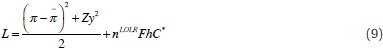
where Z is the policy weight on output variability, and F is a scaling parameter for LOLR-related costsS.20 A CB with a high value of Z is "activist" as it places a relatively high weight on reducing output volatility. Eq. (9) corresponds to the benchmark double-quadratic case. In the last term of (9), the LOLR-related component is proportional to the amount of liquidity provided and the odds -captured by h ∈(0,1) - that a bank will end up unsuccessful in its risky investment. As the funds used for LOLR transactions cannot be used for alternative purposes, unsuccessful LOLR transactions trigger opportunity costs. We abstract from the opportunity costs of successful LOLR transactions, which are normally of a short term nature, as well as from reputation costs facing the CB in the event of ultimately closing rescued banks (because there is no systematic error involved).
2.5. Unions
Wages are assumed to be bargained collectively by unions. We split the economy into M symmetric sectors (indexed by k=1,...,M). Workers of each sector are organised in a single union, so there are M unions in the economy (also indexed by k). The outcome of the wage bargaining is wk, the nominal wage (in logs). Sectoral output, yk, is given by

where η>0. In (10), we follow Cukierman and Lippi (2001), who show this specification implies that (the absolute value of) the real wage elasticity is increasing in the number of unions, M. Therefore, deviations of wk from the economy-wide wage rate induce a loss in the sector's real activity that is proportional to η. Aggregation over k in (10) gives (2).21
We model the wage bargaining process explicitly. Instead of assuming that unions base their wage decisions solely on their inflation expectations (Berlemann and Zeidler, 2009), we set up an incomplete-information game between the CB and wage setters. Within the class of games where the monetary response to wages is assumed to be uncertain to unions, we deviate from the study of a monopoly union case (Grüner, 2002), allowing for many unions as in Spyromitros and Zimmer (2009) and Sánchez (2011 and 2013).
The unions' views are formed conditional on a signal about the degree of monetary accommodation to wages. We label the expectations operator associated with the corresponding information set as Ew. Each union k sets the nominal wage to minimise expected loss22

where A measures the relative concern for the stability in real activity.
As we have mentioned, the CB is allowed to be not fully transparent. In consequence, trade unions can only partly anticipate the monetary response to their wage claims. They only know two features about the degree of monetary accommodation γ, namely, the mean Ew(γ)= _ and the variance
  . A lower is interpreted as a stricter monetary policy, while a higher σγ2 represents a stronger degree of monetary policy uncertainty. The uncertainty about parameter γ should be interpreted as arising from lack of transparency about CB preferences.
2.6. Timing
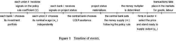
The sequence of actions comprises the following six stages (sketched in Figure 1):
-
Commercial banks collect deposits from the private sector and choose investment portfolios consisting of two projects, a risky one and a safe one.
-
All unions independently and simultaneously formulate their wage demands, conditional on a signal about the CB reaction to the economy-wide wage rate. For simplicity, it is assumed that unions know how the CB trades off overall macroeconomic stability for LOLR-related costs.
-
Commercial banks receive signals (of either high or low success) on the status of the risky project. For simplicity, it is assumed that there is no information asymmetry between banks and the CB. The CB thus also observes the signals on the projects states. Neither the comercial bank nor the CB knows at this stage whether the project will end successfully. Given that banks invest all deposits in the two projects, illiquid banks getting a low-profitability signal request LOLR assistance from the CB.
-
The CB decides which banks (if any) it assists through the discount window.
-
The CB determines the monetary base via open market opera tions.
-
Bank returns on the two investment projects materialise. Banks turn out to be solvent or insolvent. In the latter case they are closed, with the public partially moving out of deposits into cash. As a result, there is a reduction in the money multiplier and thus in the money supply. Inflation and output are determined.
3. Equilibrium Results
We solve for the equilibrium, which involves an incompleteinformation game between the CB and wage setters. In stage 1, commercial banks choose a volume of risky investment C*. Conditional on the signal they receive in stage 2, unions decide their nominal wages, trying to anticipate the monetary policy reaction in stage 5. Moreover, in stage 4 the CB decides on the provision of LOLR services, based on information about expected bank returns. We resort to backward induction, starting out with the optimisation problem of the CB.
3.1. The CB optimisation problem
The CB problem can in turn be separated in two steps: i) the CB chooses the optimal monetary base, b; and ii) the CB decides which illiquid banks it provides liquidity to.
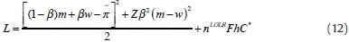
In order to compute the optimal b, let us insert Eqs. (3) and (4) for inflation and output, respectively, into the CB loss function (9), which yields:
We can then derive the optimal money supply m* by differentiating the expected loss function, EL, with respect to m and solving for m*:

where γ ≡β [Zβ[1-β)] /(1 -β)2 + Zβ2] is the degree of accommodation of monetary policy. Eq. (13) is derived taking C* and w as given.
In order to reach m*, the CB determines the monetary base. The optimal choice of b can be computed using Eq. (5) as

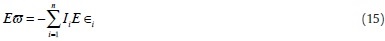
where we acknowledge that the money multiplier, ω, is uncertain. In (14), the CB forms an expectation on ω, which, from (8), equals
We calculate the optimal monetary base by plugging Eqs. (13) and (15) into (14):

Inserting Eqs. (8) and (16) into (5) gives the actual money supply:
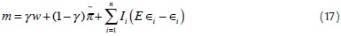
Plugging (17) into Eqs. (3) and (4), we solve for actual inflation and output as


Unexpected macroeconomic variability is here seen to be driven by bank closures, as captured by the deviations of ∈i from E ∈i. The intensity of these deviations is reflected in the variance 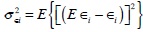 defined for each bank that is not only illiquid but also ultimately insolvent. The variance σ2∈i is linked to bank size, increasing with the number of depositors, i. e. dσ∈2i / dHi > 0.
Having thus determined the monetary base in (16), let us turn to the other CB choice, namely, which illiquid banks (if any) to assist by means of LOLR transactions. The CB decides to provide liquidity assistance if the expected loss resulting from this action is lower than when abstaining from it. The simplest way to make this comparison is to consider the CB loss stemming from any given bank i applying for LOLR help, neglecting the role played by any other illiquid bank. LOLR transactions generate a trade-off between the opportunity cost of unsuccessful liquidity assistance, FhC*, and the gain from mitigating the effect of bank closures on macroeconomic volatility.23 The loss resulting from the closure of bank i receiving LOLR services can then be expressed as24
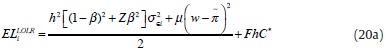
where μ≡ Zβ2/[(1-β)2 + Zβ2]∈(0,1). When the CB decides not to provide LOLR to illiquid bank i (a scenario labelled as NLOLR), the loss function does not include the term FhC*. This potential saving comes at the expense of no attempt being made by the CB at dampening macroeconomic uncertainty (i.e. bank i is closed with certainty instead of with probability h). In this case, the CB loss function thus amounts to
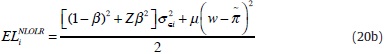
The CB provides LOLR assistance if and only if doing so leads to a total expected loss that is lower than in the case where no LOLR services are provided, that is, if and only if ELi NLOLR > ELiLOLR ⇔
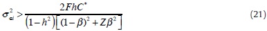
The decision to provide LOLR assistance depends on the size of the bank i via σ2∈i, which -as we have seen- rises with bank size. Intuitively, a larger depositor base causes greater uncertainty in how depositors react to the failure of bank i, thereby raising the chances of LOLR support. In contrast, small banks get no access to the discount window and are closed as soon as they face liquidity problems. This result is in line with the so-called too-big-to-fail doctrine.
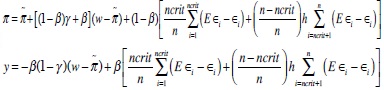
Let denote the variance which turns inequality (21) into an equality. This variance is associated with the critical bank size, i.e. the minimum size for which a bank is provided LOLR services. It is useful to sort the n illiquid banks by size such that σ2∈1 < σ2∈2 <...< σ2∈n. Thus, we end up with two different types of banks within the group of banks in liquidity troubles: small banks with σ2∈i ≤σ2crit and large banks with σ2∈i > σ2crit. Let ncrit and n-ncrit be the number of such small and large banks, respectively. A larger critical bank size is associated with a larger number of banks not being assisted by LOLR transactions (a larger ncrit). We can then rewrite the expressions for actual inflation and output in (18) and (19), respectively, as
In these two expressions, macroeconomic variability arises from unexpected fluctuations in the money multiplier. These are eliminated when there are no bank closures, in which case h = 0. (Technically, this would amount to having the critical bank size ncrit equal to zero.) For h ∈ (0,1), macroeconomic fluctuations are dampened, with some banks avoiding bankruptcy thanks to having access to LOLR services. This CB action comes on top of standard monetary policy actions via the injection of base money.
Expected CB losses can be found to equal25
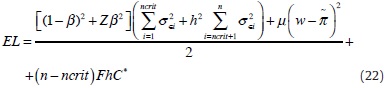
In equilibrium, the critical bank size depends on the following factors:
Proposition 1. The critical bank size is larger (smaller) and thus the number of banks not being assisted by LOLR transactions, ncrit, is larger (smaller)
i) the larger (smaller) the volume of the risky investment, C*;
ii) the larger (smaller) the probability that the risky investment fails, h;
iii) the flatter the aggregate supply curve when initially this curve is steep (flat) and the CB displays a rather strong preference for price (output) stability; or the steeper the aggregate supply curve when initially this curve is flat (steep) and the CB displays a rather strong preference for output (price) stability.
Proof. (i)[ii) It is straightforward to see that the RHS of the inequality in (21) is increasing in both C* and h. Concerning the LHS of (21), we have shown that it is increasing in bank size. Therefore, the critical bank size -obtained when (21) holds at equality- is increasing in both C* and h. This establishes items (i) and (ii).
(iii) As we have just mentioned, the critical bank size is obtained when (21) holds at equality. It depends inversely on [(1-β)2 + Zβ2] since this expression enters in the denominator of the RHS of (21). In turn, [(1-β)2 + Zβ2] is affected by β (which is an inverse measure of the aggregate supply slope) as follows:
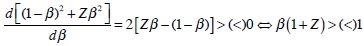
Therefore, if initially the supply curve is steep (flat) and the CB displays a stronger preference for price (output) stability -a scenario that occurs when both β and Z are low (high)- then it is likely that d[(1-β)2 + Zβ2]/ dβ < (>)0, and thus that a flatter supply curve raises (lowers) the critical bank size. QED.
Note that the initial level of the wage rate plays no role in the effects uncovered in Proposition 1, as w features in both EiLOLR and EiNLOLR with the same additive term. Therefore, wages drop out from the comparison and fail to affect the LOLR decision by the CB. In Proposition 1, the LOLR decision by the CB is affected by C*, h and β.
With regard to C* and h, these features directly raise financial costs associated with unsuccessful LOLR transactions, and they indirectly induce the critical bank size to increase (i.e. ncrit goes up). It makes sense to think that the overall effect (i.e. taking into account the policy response to adverse financial conditions) is for overall uncertainty, and thus EL, to rise with C* and h.26 Concerning β, the LOLR decision by the CB is influenced by the aggregate supply slope and thus, arguably, by trade openness.27 More specifically, a more closed economy (which is expected to display a flatter supply curve, i.e. higher β) would induce a larger (smaller) critical bank size when initially the economy is quite open (closed) and the CB displays a rather strong preference for price (output) stability. The intuition for these initial conditions is that, in an initially rather open (closed) economy output fluctuations should be relatively large (small) for any given size of inflation variability; hence, if at the same time the CB cares relatively little about price (output) stability, then the CB could afford to save less (more) banks, i.e. display a larger (smaller) critical bank size.
3.2. The Unions' Problem
Let us turn to the wage setting problem. All unions independently and simultaneously set their nominal wage, trying to minimise (11) taking into account the expressions for inflation in (18) and sectoral output in (10), as well as the expected CB reaction from (17). Optimisation implies that, in the symmetric equilibrium, the aggregate nominal wage equals28
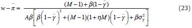
which is positive when unions are non-atomistic (M<∞), but vanishes (i.e. wages approach their competitive level) as unions become atomistic (M→∞). Use of (23) leads to the following result:
Proposition 2. If unions are non-atomistic (M<∞), the aggregate nominal wage
i) decreases with monetary policy uncertainty, σ2γ;
ii) decreases (increases) with the degree of monetary policy strictness -as given by a smaller γ - when CB policies are initially seen as rather strict (accommodating) and transparent (opaque);
iii) decreases (increases) with the number of unions, M, and thus increases (decreases) with the degree of wage bargaining centralisation, when CB policies are initially seen as rather strict (accommodating) and transparent (opaque).
As unions become atomistic (M→∞) all of these wage effects vanish.
Proof. (i) Differentiation of (23) with respect to σ2γ yields
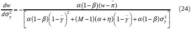
If M<∞, the nominal wage clearly falls as a result of larger monetary uncertainty. Intuitively, a larger value of σ2γ renders monetary policies more unpredictable, inducing unions to moderate their wage claims.
(ii) Differentiation of (23) with respect to gives
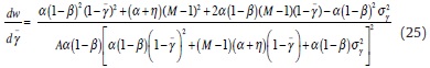
If M<∞, by inspecting the numerator, dw / d is more likely to be positive (negative) under two initial conditions: i) when is small (large) and thus (1 - ) large (small), and ii) when σ2γ is small (large). This establishes (ii), as it implies that dw / d > (<)0, i.e. w decreases (increases) with a smaller -which characterises a tighter policy rule- when the CB is initially known to be rather strict (accommodating) and transparent (opaque). Intuitively, when the CB is seen as non-accommodating and monetary uncertainty is low (i.e. for low values of and σ2γ), a stricter monetary regime elicits wage restraint on the part of unions. The opposite effect is induced by a fall in when monetary policies are known to be rather accommodating and opaque (i.e. for high values of and σ2γ). Under these initial conditions the deterrence exerted on unions is undermined, with tighter monetary policymaking ultimately raising w.
(iii) Differentiate (23) with respect to M to get
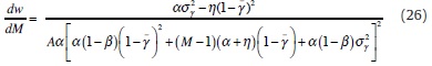
If M<∞, inspection of the numerator shows that dw / dM is more likely to be negative (positive) when initially is small (large) and σ2γ is small (large). Therefore, it is more likely that dw / dM <(>)0, i.e. w decreases (increases) with a larger M -which indicates a lower degree of wage bargaining centralisation- when the CB is initially known to be rather strict (accommodating) and transparent (opaque). This establishes (iii). Intuitively, there are two forces at play here. First, more unions means that each of them internalises less of the impact that individual wage claims exert on the macroeconomy. As a result of this free riding, wages tend to increase, as given by an increase in the numerator of (21). Second, more unions also means that the denominator of (21) rises because of the increased competition among unions. This makes w go down, as each union becomes more concerned consequences of individual wage demands for real activity. For instance, one gets that dw / dM <0 when the denominator of (21) rises by more than the numerator, which occurs when the increased competition arising from a larger M outweighs the free riding effect also involved. From (26), this turns out to be the case when monetary policies are perceived as non-accommodating and predictable (i.e. for low values of and σ2γ).
Finally, as unions become atomistic (M→∞) the wage effects in Eqs. (24) through (26) go to zero. Atomistic unions are not at all concerned about the consequences of their individual wage demands on the macroeconomy, irrespective of the values adopted by monetary policymaking parameters and σ2γ. QED.
With regard to item (iii) in Proposition 2, the present model can be seen as encompassing two earlier studies, namely, those of Cukierman and Lippi (2001) and Grüner et al. (2009). Under full CB transparency (i.e. σ2γ=0), we reproduce Cukierman and Lippi's (2001) result that a less centralised wage bargaining (higher M) reduce nominal wages owing to unions' fear that high wages will lead to increased unemployment owing to greater competition among workers. Grüner et al. (2009) instead allow for imperfect CB transparency, while abstracting from labour competition (i.e. η=0). We reproduce the two possible cases considered by Grüner et al. (2009): i) under full CB transparency (i.e. σ2γ=0), decentralisation in wage bargaining has no effect on w;29 and ii) under incomplete CB transparency (i.e. σ2γ>0), decentralisation in wage bargaining raises nominal wages as each (now smaller) union internalises to a lesser extent the adverse consequences that higher wage claims exert on sectoral output. Compared with these two earlier studies, our derivations present the advantage of a general formulation, also including the case when CB transparency is imperfect (i.e. σ2γ>0) and there is competition between different unions' workers (i.e. η>0).
In addition, the result in item (iii) indicates that the effect of wage bargaining centralisation on wages depends on the nature of monetary institutions. When unions perceive CB policies as rather strict and transparent, wages are lower with less centralised wage bargaining (higher M). In contrast, when CB policies as seen rather accommodating and opaque, a fall in w is induced not by higher competition among unions but by more centralised wage bargaining (lower M). The latter is associated with more cautious behaviour on the part of unions, each of which internalises to a greater extent the macroeconomic consequences of its wage claims.
Finally, it is worth elaborating on one aspect of items (ii) and (iii) in Proposition 2. These items refer to two initial conditions, namely, the monetary authority' conservativeness and transparency. While there is no clear upper-bound on CB's unpredictability. it has been argued that there may be a lower bound on σ2γ. This is the case of Cukierman's (2009) discussion about the so-called "limits of transparency". These are supposed to reflect constraints on how much the monetary authority knows about the actual level of the output gap and about the impact of policy on inflationary expectations. If the lower bound for σ2γ is large enough (i.e. if CB transparency cannot be too high), then Proposition 2 would be relevant only in case greater monetary strictness (lower ) and less centralised wage bargaining (higher M) raise nominal wages. Otherwise, there would be scope for the fully non-linear (threshold) results contained in Proposition 2.
3.3. Enhancing Macroeconomic and Financial Stability
We assume that the loss function of the CB is formally the same as that of society. Therefore, (22) equals expected losses for both the CB and society. We thus abstract from aspects that would imply a difference between the two. Such aspects may include optimal delegation à la Rogoff (1985), whereby the CB should be more conservative than society, or the type of CB approach advocated by Blinder (1997) to eliminate the inflation bias, which involves a CB target for unemployment above its socially optimal level.
As we have seen, social losses are expected to rise in the event of adverse exogenous financial developments, as given by a rise in financial assistance costs (higher C* and h), or a reassessment by households of deposit risks leading to an upward shift in the distribution of the σ2∈i's. In response to these developments, the CB would reduce the scope of its LOLR services. Put it differently, the critical bank size used to decide LOLR assistance would go up (i.e. a higher ncrit). Although this action reduces the cost associated with LOLR transactions, overall social losses would normally rise.
If the initial equilibrium were fully efficient, there would simply be no scope for improvement. In our model the equilibrium reflects noncooperative actions concerning the interaction between unions and the CB. Labour market outcomes thus deviate from the efficient solution. In the case of CB transparency, it could the case that it is set at an inefficiently high level owing to international benchmarking or domestic regulation (e.g. because inflation targeting involves this as a requirement). Initial deviations from efficiency motivate our interest in the role played by policy actions in dampening social losses.
In this regard, let us look at the inefficiency in the labour market. Inspection of (22) indicates that the wage premium over its competitive level is socially costly. Therefore, the factors pushing wages down in Proposition 2 contribute to a more efficient outcome, helping offset to a certain extent the loss arising from the financial shock. From this particular angle, we can derive the following conclusions:
Proposition 3. Macroeconomic stability is higher
i) the more opaque the CB (higher σ2γ);
ii) the greater (smaller) the degree of monetary policy accommodation,
iii) the smaller (greater) the number of unions, M, and thus the greater (smaller) the degree of wage bargaining centralisation when CB policies are initially seen as rather strict (accommodating) and transparent (opaque).
As unions become atomistic (M→∞) all of these wage effects vanish.
Proof. From (22), the wage premium over its competitive level is socially costly, i.e. dEL / dw>0. Based on this together with the results in Proposition 2 concerning the parameters of interest (namely, σ2γ, and M), it is straightforward to derive the results in Proposition 3. QED.
Proposition 3 refers to macroeconomic stability in terms of an ex-ante performance evaluation. As such, it concerns the unconditional expectation of variability arising from money demand disturbances. This Proposition need not hold ex-post, i.e. for the actual realisation of shocks at a given point in time.
In addition to wage developments, it is also worth considering the role of the supply curve slope (which may be influenced by trade openness) for macroeconomic and financial stability. It is found that the impact of β on EL is relatively complex. A change in the supply curve slope affects wages in complicated ways -see Eq. (23)-, on top of raising the coefficient m premultiplying  in (22). Moreover, β has ambiguous consequences for stability via the number of banks not assisted by LOLR transactions, ncrit. This is so both because β influences ncrit in a way that is parameter-dependent (see Proposition 1) and because ncrit itself has two effects which are overall ambiguous. First, it lowers the financial costs relating to LOLR transactions, given by (n - ncrit)FhC*. Second, as long as LOLR transactions need not be successful (i.e. for h ∈(0,1) ), ncrit raises
  in (22), as fewer banks receive LOLR assistance.30 All in all, it is not possible to derive an unequivocal role of β for macroeconomic and financial stability, as the effects described in this paragraph point in various possible directions. Given the complexity involved in the effects of the supply curve slope (which may be affected by trade openness) on EL, policymakers might want to abstain from influencing β unless they have a clear idea of the structural parameters of the model.
3.5. Role of Moral Hazard
In the absence of moral hazard, we have seen that only the largest banks receive LOLR assistance. LOLR services are often seen as leading to moral hazard behaviour on the part of commercial banks. In the present modelling context, Berlemann and Zeidler (2009) analyse the effects of moral hazard behaviour, considering the roles of both the expected profit of banks and the optimal amount of capital thay they invest into the risky project. These authors show that the largest banks react to the provision of LOLR services by increasing their risky exposures. Berlemann and Zeidler (2009) also show that, concerning the remaining banks (i.e. the "small" and "very small"), those in the former group have an incentive to decrease their investments into risky projects in order to get access to LOLR transactions. It is only the "very small" banks that do not alter their behaviour when LOLR is provided by the CB and thus display no moral hazard behaviour. In equilibrium banks' responses to (a larger) LOLR provision contribute to lower inflation and output variability but also higher costs associated with financial assistance.31 The overall effect on EL is thus ambiguous, with macroeconomic stability pushing CB losses down as financial costs push them up.
Our introduction of unionised wage setting into the analysis does not affect the previous results on moral hazard. But wage setting considerations are worth considering with regard to the implications of moral hazard for CB losses. First of all, given that the overall effect of moral hazard on EL is ambiguous, in case CB losses rise the authorities could consider institutional changes that lead to wage discipline in an attempt to keep macroeconomic performance under check. Second, the results described in the previous paragraph assume that the CB has access to the additional financial resources derived from moral hazard. If the CB lacks the funds needed to dampen macroeconomic instability, this would be another reason for the policymakers to adjust economic institutions so as to reduce the premium of wages over their competitive level.
Going beyond the present modelling environment, the literature has studied cases where LOLR services may have different implications for moral hazard. As we have seen, Berlemann and Zeidler (2009) show that, under moral hazard behaviour, relatively large banks react by increasing their risky investments. In contrast, Perotti and Suárez (2002) argue that moral hazard implies that it is smaller banks that would be willing to take greater risks, while larger banks would proceed more cautiously. Among other studies, Repullo (2011) shows that LOLR does not increase the incentives to take risk, while insufficient capital requirements and penalty interest rates charged for liquidity assistance do. Freixas et al. (2004) find that LOLR has different implications for the efficiency of an unsecured interbank market depending on the source of moral hazard.
4. Conclusions
We introduce imperfect monetary policy transparency and strategic wage setting into a macro model where the CB provides LOLR services to banks on top of its standard stabilisation policy. The CB provides liquidity assistance to illiquid commercial banks with the aim that these banks avoid bankrupcy. Whenever banks are closed there are wider fluctuations in the money multiplier (and thus in inflation and output), which makes monetary policy more difficult and causes welfare decreasing fluctuations of inflation and output around their target levels.
At a given point in time, the equilibrium of a given economy may be characterised by coordination failure. The occurrence of major shocks (such as those behind the latest financial crisis) may offer the opportunity for institutional reform that tackles both the latest disturbance and the existing coordination problem. In addition, policymakers' behaviour, which may in "normal" times face binding constraints, e.g. from regulation or benchmarking, might change in the light of exceptional circumstances. Against this background, the present paper studies how the trade-off between financial instability and macroeconomic variability can be improved by adjustments in the economic structure (possibly influenced by trade openness) and institutions (as given by the monetary policy setup, wage bargaining and the non-cooperative game involved between the CB and wage setters). This comes on top of the CB policy decisions concerning standard monetary policy and LOLR transactions, also considered in this paper. It is also different from the roles of the CB in bank supervision and macroprudential regulation, which could be seen as attempting to tackle the trade-off between moral hazard and bailout uncertainty (Cukierman, 2013).
The main results obtained here are the following. In a context of costly LOLR transactions, the CB has an incentive to save only large banks, a well-documented empirical phenomenon known as "too-big-to-fail doctrine". CB opaqueness can help improve macroeconomic stability by making wages closer to their competitive levels. In contrast to this role for opaqueness about CB preferences, it is best for the CB to reveal its LOLR transactions so as to avoid excessive macroeconomic instability. Turning to monetary policy accommodation and wage bargaining centralisation, these factors may help discipline wages and thus improve stability when CB policies are initially seen as rather strict and transparent. The role of the supply curve slope (which may be affected by trade openness) is relatively complex, so policymakers might want to abstain from influencing it unless they have a clear idea of the structural parameters of the model. This means that, even if the economy falls in a recession amidst financial uncertainty, we advocate a cautious approach regarding international trade. The reasons given here differ from the position that, in the absence of international coordination, protectionism may lead to retaliation and risk bringing global trade down.
Concerning the role of wages in the model, two clarifications are in order. First, the result that lower wages are more efficient in part reflects the fact that the model used here represents the supply side in much more detail than the demand side. In a recessionary context, it may be realistic to allow wage restraint to play some role in pushing aggregate demand down.32 Second, wages are found not to influence the critical bank size involved in LOLR decisions. This could be seen as arising from our use of double-quadratic preferences for the CB. It may be worth examining if wages could affect the critical bank size in case a different functional form for the CB loss function were used (such as the asymmetric specifications advocated by Cukierman and Gerlach, 2003, or Goodhart, 1999).
We have also considered the implications of moral hazard within the model.33 The moral hazard results obtained by Berlemann and Zeidler (2009) are found to still hold in a more realistic wage setting environment. Moral hazard then leads to more bank rescues than in the case where no moral hazard is present. Ex-post, more banks will be saved, which induces higher macroeconomic stability at the expense of increased LOLR-related costs. The overall effect of moral hazard on CB losses is thus ambiguous. From the angle of unionised wage setting, we add the following two results regarding the implications of moral hazard for CB losses. First, in case CB losses rise the authorities could still consider institutional changes that enhance wage discipline in an attempt to dampen macroeconomic instability. Second, if the CB lacks the financial resources required in the present situation, policymakers may also opt for adjusting the institutional setup with the aim of reducing labour market distortions.
Given the simplicity of the framework adopted, the analysis has to acknowledge a number of limitations. For instance, the returns of the risky investment could be made dependent on the decisions of unions and firms. Moreover, wage setting arrangements here impact CB losses via their effects on macroeconomic variables, not in connection with financial stability considerations (e.g. via the CB decisions as to which and how many banks to save). The issues of financial stability and macroprudential regulation are beyond the scope of the present paper. Addressing them would necessitate other model extensions, such as the ones that follow. First, it could introduce an interbank market to compare LOLR and standard liquidity facilities provided by CBs. Second, unions could be made sensitive to financial distress as firms may become liquidity-constrained, affecting the unions' objective function. Third, moral hazard issues could be made more realistic by allowing not just the volume of loans to be endogenous to the LOLR policy, but also bank size (i.e. the deposit base). Fourth, the CB may be allowed to have a different information set from that available to individual banks; monitoring issues and information disclosure could then be discussed in relation with LOLR operations.
Acknowledgements
We gratefully thank David Marqués Ibáñez for helpful discussions and an anonymous referee for valuable comments. Views expressed are not necesarily those of the European Central Bank. Any remaining errors are the responsibility of the author.
Notes
1Even prior to the latest crisis, there is empirical evidence of LOLR transactions from a wide variety of experiences (Bordo, 1986; Dowd, 1999; Eichengreen and Portes, 1987; Humphrey and Keleher, 1984).
2There have been changes in the institutional arrangements for handling financial crises. While CBs tackled such crises in most countries largely on their own, crises are becoming increasingly managed by a committee of public sector agencies. Thus far, the literature has not addressed the challenge of formally modelling such a development.
3vMoral hazard is a standard feature in models of bank behaviour. Moral hazard arises in the presence of informational frictions and 'agency problems' between bank managers and owners (Gorton and Rosen, 1995). Better capitalised banks have less moral hazard incentives (Jeitschko and Jeung, 2005) and are more prone to adopt careful practices to reduce costs. Regulators can force banks to increase the amount of capital commensurably with the amount of risk taken (Gropp and Heider, 2010). Hellman et al. (2000) argue that banks could also respond to regulatory actions forcing them to hold more capital by increasing portfolio risk.
4For an alternative approach, see Cordella and Levy Yeyati (2003).
5The presence of learning distinguishes Bianchi et al. (2012) from studies assuming that agents form rational expectations with full information, such as Benigno et al. (2013), Bianchi (2011), Bianchi and Mendoza (2010), Jeanne and Korinek (2010), Korinek (2013), Lorenzoni (2008), and Stein (2012). Concerning the role of credit frictions and imperfect information, Bianchi et al. (2012) relate to the financial accelerator models of Aiyagari and Gertler (1999), Bernanke et al. (1999), and Kiyotaki and Moore (1997).
6As large banks have a higher chance of being saved, this may trigger bank mergers, implying lower funding cost (Hunter and Wall, 1989; Boyd and Graham, 1991; Benson et al., 1995; Penas and Unal, 2004; DeYoung et al., 2009, and Rose and Wieladek, 2012). Another rationale for large bank size is inadequate corporate governance enabling bank managers to pursue high-growth strategies at the expense of shareholders. In the latest crisis, the too-big-to-fail argument may have been mitigated by the severe deterioration in the public finances, which reduces countries' ability to guarantee bank liabilities and makes large banks subject to greater market discipline (Demirguc-Kunt and Huizinga, 2013a and 2013b; see also Acharya et al., 2013).
7The general issue of the role of coordination failure for the performance of institutional reform is discussed in Fanelli (2007).
8In a context of "liquidity trap", the role of base money (which underlies the concept of money multiplier) can be rationalised by the standard argument that money is a better indicator of monetary policy stance than the interest rate. In more normal times, there should be an inverse relation between interest rates and money supply.
9Berlemann and Zeidler (2009) do not include an output objective in the CB loss function.
10Sánchez (2008) uses this feature of the Phillips curve within a simple model. This feature conveys an open economy flavour, even if ours is a closed economy model. To some extent a similar interpretation can be applied to the assumption that, following a bank closure, the public suddenly changes its preferences towards holding domestic currency. Although we abstract from the possibility that depositors switch out of the deposits of banks perceived as risky into foreign exchange, as has occurred in the financial crises of Mexico (1995), Asia (1997-1998), Russia (1998), and Argentina (2000-2001), we are able to capture the partial aspect of financial disintermediation triggered by the banking panic.
11Since this is a static model we use inflation π interchangeably with the price level (in logs), resorting to the normalisation that the previous period's price level is zero.
12To derive (3) and (4), first plug (2) into (1) to get π =(m +αw) /1+α) , which -using the definition of β- yields (3). Eq. (4) can be derived by inserting (3) into (2), which gives y = α (1-β)(m - w); given that the definition of β implies that α (1-β)= β, then y can be expressed as in (4).
13This simplified formulation could be derived by assuming decreasing marginal returns for each loan to non-banking firms, in conjunction with an exogenous allocation of loans across banks. A more general model would allow for credit demand considerations, endogenising the allocation of loans across banks (see Schnabl, 2012).
14Since it is not the aim of this paper to explain the structure of the banking sector we stick to the assumption that bank sizes are given exogenously.
15The signal Xi is directly related to the actual realisation of the bank-specific variable λi, which is the only random element weighing on the return of the risky investment, Ci.
16The CB has the information needed to judge whether there is a risk that a commercial bank's profits be insufficient to meet all its liabilities, in which case the bank may be supported with LOLR credit. Healthy banks are never supported by LOLR transactions, given that these are assumed to be only aimed at preventing uncertainty on the money multiplier.
17This can be justified by supposing that depositors are identical in their financial wealth and preferences towards cash and deposits.
18As we saw earlier, when a bank is closed the remaining funds of the bank are evenly distributed among its depositor base. For the remainder of the money deposited, depositors are also assumed to get it back from insolvent banks. As with Berlemann and Zeidler (2009), we abstract from other details and consequences concerning the deposit insurance scheme involved.
19We shall later show how the number of banks receiving help, nLOLR, is determined. For nLOLR to make sense, the number and size of the banks in trouble that are supported must keep some proportion with overall economic activity and the amount of CB financial resources available (both for assisting banks and for insuring deposits in the event of bankrupcies). Another exogenous parameter, n, can only make sense under similar conditions.
20As mentioned above, the additional capital provided by LOLR assistance is a fraction of the capital already invested in the project, C*. F is the policy weight on costly LOLR transactions (relative to macroeconomic instability).
21To see this, aggregate over k in (10) to get  Given that
  , y is found to be the same as in (2). k=1
22We use y2k instead of a squared unemployment term, as is standard in the related literature. These two variables are known to be proportional under the widely maintained assumptions of a fixed labour supply and labour being the only variable input.
23Technically, the relevant expected CB losses can be computed by substituting the impact exerted by a given bank i on objective function (12) via Eqs. (18) and (19). Stochastic macroeconomic volatility is driven by the last term in both Eqs. (18) and (19).
24See derivation in Appendix A.
25See derivation in Appendix A.
26An effect similar to those of C* and h would arise if the distribution of the σ2 ∈i 's shifted upwards, i.e. if households were to consider it riskier to keep deposits at their banks in the event the latter have to be closed.
27Under asymmetric CB objective functions, the range of macroeconomic factors weighing on the critical bank size will be expanded to include monetary policy parameters.
28See derivation in Appendix A.
29The difference vis-à-vis Cukierman and Lippi (2001) resides in the role that the latter assign to labour competition (i.e. η>0), which is switched off by Grüner et al. (2009).
30To make things more complicated, the factor is premultiplied by [(1-β)2 + Zβ2] which depends in an ambiguous manner on β.
31This stems from two effects. First, the largest banks receive more LOLR assistance when they engage in moral hazard behaviour. Second, there is a larger number of banks being provided with financial support. Some of the LOLR services do not succeed in saving the ailing banks, which leads to rising overall costs from LOLR transactions.
32The lack of detail concerning demand also means that the study is unable to assess the role of product market competition (and thus the effects of product market reform).
33Although LOLR services are often seen as leading to serious moral hazard behaviour on the side of commercial banks, it is not clear from the literature how smaller and larger banks modify risk-taking behaviour in reaction to the provision of LOLR services.
References
Acharya, V., Drechsler, I., Schnabl, P. (2013). A Pyrrhic Victory? - Bank Bailouts and Sovereign Credit Risk. Journal of Finance (forthcoming). [ Links ]
Aiyagari, R., Gertler, M. (1999). Overreaction of Asset Prices in General Equilibrium. Review of Economic Dynamics 2, 3-35. [ Links ]
Benigno, G., Chen, H., Otrok, C., Rebucci, A., Young, E. (2013). Financial Crises and Macro-Prudential Policy. Journal of International Economics 89, 453-470. [ Links ]
Benson, G., Hunter, W., Wall L. (1995). Motivations for bank mergers and acquisitions: enhancing the deposit insurance put option versus earnings diversification. Journal of Money, Credit and Banking 27, 777-788. [ Links ]
Berlemann, M., Zeidler, M. (2009). The macroeconomics of lending of last resort: A positive perspective. Jahrbucher für Wirtschaftswissenschaften 59, 209-225. [ Links ]
Bernanke, B., Gertler, M., Gilchrist, S. (1999). The financial accelerator in a quantitative business cycle model. In: Taylor, J., Woodford, M. (Eds.), Handbook of Macroeconomics, vol. 1C, North-Holland. [ Links ]
Bianchi, J. (2011). Overborrowing and Systemic Externalities in the Business Cycle. American Economic Review 101, 3400-3426. [ Links ]
Bianchi, J., Mendoza, E. (2010). Overborrowing, Financial Crises and 'Macroprudential' Policy. NBER Working Paper No. 16091. [ Links ]
Bianchi, J., Boz, E., and Mendoza, E. (2012). Macroprudential Policy in a Fisherian Model of Financial Innovation. IMF Economic Review 60, 223-269. [ Links ]
Blanchard, O., Romer, D., Spence, M., Stiglitz, J. (Eds.) (2012). In the Wake of the Crisis: Leading Economists Reassess Economic Policy. MIT Press, Cambridge. [ Links ]
Blinder, A. (1997). What central bankers could learn from academics - and vice-versa. Journal of Economic Perspectives 11, 3-19. [ Links ]
Bordo, M. (1986). Financial crises, banking crises, stock market crashes and the money supply: Some international evidence, 1887-1933. In: Capie, F., Wood, G. (Eds.), Financial Crises and the World Banking System. MacMillan, London. [ Links ]
Boyd, J., Graham, S. (1991). Investigating the bank consolidation trend. Federal Reserve Bank of Minneapolis Quarterly Review, Spring, 1-15. [ Links ]
Cordella, T., Levy Yeyati, E. (2003). Bank bailouts: moral hazard vs. value effect. Journal of Financial Intermediation 12, 300-330. [ Links ]
Cukierman, A., Lippi, F. (2001). Labor markets and monetary union: A strategic analysis. The Economic Journal, 111, 541-565. [ Links ]
Cukierman, A. (2009). The limits of transparency. Economic Notes 38, 1-37. [ Links ]
Cukierman, A. (2013). Monetary policy and institutions before, during, and after the global financial crisis. Journal of Financial Stability 9, 373-384. [ Links ]
Demirguc-Kunt, A., Huizinga, H. (2013a). Are banks too big to fail or too big to save? International evidence from equity prices and CDS spreads. Journal of Banking & Finance 37, 875-894. [ Links ]
Demirguc-Kunt, A., Huizinga, H. (2013b). Do we need big banks? Evidence on performance, strategy and market discipline. Journal of Financial Intermediation (forthcoming). [ Links ]
DeYoung, R., Douglas, E., Molyneux, P. (2009). Mergers and acquisitions of financial institutions: a review of the post-2000 literature. Journal of Financial Services Research 36, 87-110. [ Links ]
Diamond, D., Dybvig, P. (1983). Bank runs, deposit insurance, and liquidity. Journal of Political Economy 91, 401-419. [ Links ]
Dowd, K. (1999). Too big to fail? Long-Term Capital Management and the Federal Reserve. Cato Institute Briefing Paper No 52, Washington D.C. [ Links ]
Eichengreen, B., Portes, R. (1987). The anatomy of financial crises. In: Portes, R., Swoboda, A. (Eds.), Threats to international financial stability. Cambridge University Press, New York. [ Links ]
Fanelli, J. (2007). Structural Reform and Macroeconomics. In: Heymann, D. (Ed.) Advances in Macroeconomics (in Spanish). Editorial Temas-AAEP, Buenos Aires. [ Links ]
Freixas, X., Parigi, B. (2012). Lender of Last Resort and Bank Closure Policy. In: Berger, A., Molyneux, P., Wilson, J. (Eds.), The Oxford Handbook of Banking. Oxford Handbooks Online, Oxford. [ Links ]
Freixas, X., Parigi, B., Rochet, J.-C. (2004). The Lender of Last Resort: A Twenty-First Century Approach. Journal of European Economic Association 2, 1085-1115. [ Links ]
Goodfriend, M. King, R. (1988). Financial Deregulation Monetary Policy and Central Banking. In: Haraf, W., Kushmeider, R. (Eds.), Restructuring Banking and Financial Services in America. American Enterprise Institute, Washington. [ Links ]
Goodhart, C. (1999). Central bankers and uncertainty. Bank of England Quarterly Bulletin 39, 102-121. [ Links ]
Goodhart, C., Huang, H. (2005). The lender of last resort. Journal of Banking & Finance 29, 1059-1082. [ Links ]
Gorton, G., Rosen, R. (1995). Corporate control, portfolio choice and the decline of banking. Journal of Finance 50, 1377-1420. [ Links ]
Gropp, R., Heider, F. (2010). The determinants of bank capital structure. Review of Finance 14, 587-622. [ Links ]
Grüner, H. (2002). How Much Should Central Banks Talk? A New Argument. Economics Letters 77, 195-198. [ Links ]
Grüner, H., Hayo, B., Hefeker, C. (2009). Unions, Wage Setting and Monetary Policy Uncertainty. The B.E. Journal of Macroeconomics, Topics 9, Article 40. [ Links ]
Hellmann, T., Murdock, K., Stiglitz, J. (2000). Liberalization, moral hazard in banking, and prudential regulation: Are capital requirements enough? American Economic Review 90, 147-165. [ Links ]
Humphrey, T., Keleher, R. (1984). The lender of last resort: A historical perspective. Cato Journal 4, 275-318. [ Links ]
Hunter, W., Wall, L. (1989). Bank merger motivations: A review of the evidence and an examination of key target bank characteristics. Federal Reserve Bank of Atlanta Economic Review 74, 2-19. [ Links ]
Jeanne, O., Korinek, A. (2010). Managing Credit Booms and Busts: A Pigouvian Taxation Approach. NBER Working Paper No 16377. [ Links ]
Jeitschko, T., Jeung, S. (2005). Incentives for risk-taking in banking: A unified approach. Journal of Banking and Finance 29, 759-777. [ Links ]
Kiyotaki, N., Moore, J. (1997). Credit Cycles. Journal of Political Economy 105, 211-248. [ Links ]
Korinek, A. (2013). Systemic Risk-Taking: Accelerator Effects, Externalities, and Regulatory Responses. Review of Economic Studies (forthcoming). [ Links ]
Lorenzoni, G. (2008). Inefficient Credit Booms. Review of Economic Studies 75, 809-833. [ Links ]
McAndrews, J., Potter, S. (2002). Liquidity effects of the events of September 11, 2001. Federal Reserve Bank of New York Economic Policy Review 8, 59-79. [ Links ]
Penas, M., Unal, H. (2004). Too-Big-To-Fail Gains in Bank Mergers. Evidence from the Bond Market. Journal of Financial Economics 74, 149-179. [ Links ]
Perotti, E., Suárez, J. (2002). Last bank standing: What do I gain if you fail? European Economic Review 46, 1599-1622. [ Links ]
Repullo, R. (2011). Liquidity, Risk Taking, and the Lender of Last Resort. In: Allen, F., Carletti, E., Krahnen, E., Tyrell, M. (Eds.), Liquidity and Crises. Oxford University Press, Oxford. ch. 11. [ Links ]
Rochet, J.-C., Vives, X. (2004). Coordination Failures and the Lender of Last Resort: Was Bagehot Right After All? Journal of the European Economic Association 2, 1116-1147. [ Links ]
Rogoff, K. (1985). The optimal degree of commitment to an intermediate monetary target. Quarterly Journal of Economics 100, 1169-1189. [ Links ]
Romer, D. (1993). Openness and Inflation: Theory and Evidence. Quarterly Journal of Economics 108, 869-903. [ Links ]
Rose, A., Wieladek, T. (2012). Too big to fail: Some empirical evidence on the causes and consequences of public banking interventions in the UK. Journal of International Money and Finance 31, 2038-2051. [ Links ]
Sánchez, M. (2008). Implications of monetary union for catching-up member states. Open Economies Review 19, 371-390. [ Links ]
Sánchez, M. (2011). Monetary strictness and labour market outcomes under incomplete transparency. Research in Economics 65, 95-99. [ Links ]
Sánchez, M. (2012). Inflation uncertainty and unemployment uncertainty: Why transparency about monetary policy targets matters. Economics Letters 117, 119-122. [ Links ]
Sánchez, M. (2013). Monetary accommodation, imperfect central bank transparency and optimal delegation. Economics Letters 120, 392-396. [ Links ]
Schnabl, P. (2012). The International Transmission of Bank Liquidity Shocks: Evidence from an Emerging Market. Journal of Finance 67, 897-932. [ Links ]
Spyromitros, E., Zimmer, B. (2009). Monetary accommodation and unemployment: Why central bank transparency matters. Economics Letters 102, 119-121. [ Links ]
Stein, J. (2012). Monetary policy as financial-stability regulation. The Quarterly Journal of Economics 127, 57-95. [ Links ]
