


 English (pdf)
 Article in xml format
 Article references
 Send this article by e-mail
 Cited by SciELO
  Cited by Google
  Similars in
SciELO
Similars in
SciELO  Similars in Google
 Permalink
1. Introduction
Forecasts constitute a tool of great importance within the process of operations planning. As simple as the methods to meet this end might be, the decisions made outside these techniques are quite few since these provide the information necessary to know with relative exactitude the events on which an action course must be taken. From this perspective, decisions related to optimizing physical spaces, operations’ speed, redesigning processes, financial performance improvement, products design and development, human talent wellbeing, long term stability, environment, productivity and competitiveness require a forecast (Krajewski, Ritzman and Malhotra, 2008; Vollmann, Berry, Whybark and Jacobs, 2005 and Martinich, 1997).
Within this context, this paper’s development initially comprehends the theoretical structure by which this study is supported and highlights the importance of forecasts in organizations. Likewise, the most important traits of the binomial logistic regression model will be highlighted, which permits to classify the companies analyzed in one of the subgroups established by the two values of the dependent variable, namely, whether these companies perform forecasts or not. Afterwards, the methodology guiding this research will be presented in order to stablish the variables influencing businessmen’s choice to use different prediction tools, which constitutes the work’s objective. Lastly, the discussion of the results and conclusions are presented.
2. Theoretical framework
2.1. Forecasts
According to Martinich (1997), prognoses are “the art and the science of predicting future events” (p. 102). The most important organization decisions are on the exactitude of these techniques (Greasley, 2009; Sanders and Gramanb, 2009; Bermúdez, et al., 2006; Makridakis, Michele and Moser, 1978). Likewise, the prognosticator’s training Mentzer and Cox, 1984; Winklhofer, Diamantopoulus and Witt, 1996; Sanders, 1992), the usage of combined prognoses (Winkler and Makridakis 1983; Fildes, 1989; Bunn and Vassilopoulus, 1999) and employing consultants (Winklhofer et al., 1996; Vonderembse and White, 2004) have a direct effect on the predictions’ exactitude.
Applying prognoses significantly contributes, among other aspects, to inventory optimization (Mentzer and Schroeter, 1994; Moon, Mentzer, Smith and Graver, 1998; Sanders, 1992; Fildes, Nikolopoulos, Crone and Syntetos, 2008) and to efficiency in the processes of strategic planning (Finney, 2012; Mentzer and Cox, 1984; Li, Cheng and Gray, 1999; Power, 1995; Sanders, 1992; Oliva and Watson, 2012; Hogarth and Makridakis, 1981; Herbig, Milewicz and Golden, 1993), which aims at improving organizational performance (Nahmias, 2007; Krajewski, Ritzman and Malhotra, 2010; Meredith and Shafer, 2010; Chen and Guo, 2011).
Within this context, organizations currently perform in a turbulent, chaotic and unpredictable environment where managing the environment’s information (Genç, Alayoğlu and Iyigün, 2012; Stone and Fiorito, 1986; Finney, 2012; Oliva and Watson, 2012; Raspin & Terjesen, 2007; Hogarth and Makridakis, 1981; Daniells, 1981; Herbig et al., 1993; Winklhofer et al., 1996) is a critical aspect in the practice of organizational forecasting.
Companies’ internal information (Genç et al., 2012; Oliva and Watson, 2012), technology (Russell and Taylor, 1995; Reid and Sanders, 2010; Schroeder, Meyer and Rungtusanatham, 2011; Krajewski et al, 2010; Heizer and Render, 2011; Meredith and Shafer, 2010), organizational communication (Oliva and Watson, 2012; Mintzberg, Brian and Voyer, 1997), incentives to workers, (Oliva and Watson, 2012), team work (Winklhofer et al., 1996), employees’ participation in decision making (Robbins and Coulter, 2010; Dess, Lumpkin and Eisner, 2011; Russell and Taylor, 1995) and the periodicity in which predictions are performed (Russell and Taylor, 1995, Mentzer and Schroeter, 1994; Schroeder et al., 2011; Winklhofer et al., 1996; Herbig et al., 1993) are deemed as fundamental elements to perform prognoses.
2.2 Logistic Regression
Logistic regression is an explanatory method of inferential statistics (Martín, Cabero and de Paz, 2008, p.272). This technique seeks to attain a lineal function of the independent variables that allows to classify individuals in one of two sub-populations or groups established by the two values of the dependent variable (Ferrán, 2001, p. 232; Hair, Anderson, Tatham and Black, 1999). According to Guisande, Vaamonde and Barreiro (2011) regression models for qualitative dependent variables, allows to evaluate the influence of independent variables over the dependent variable, giving a probability as a result (p. 537) (Martín et al., 2008).
Just as with quantitative dependent variables regression it’s necessary for multicollinearity not to exist between the different independent variables and the observations of the sample must be independent inwardly. In this case, it’s not required for the residue to bear a normal distribution, nor the homoscedasticity hypothesis (constant variance of the residue) (Guisande, et al., 2011, p. 537; Pérez, 2009). According to Hair et al. (1999):
Logistic regression, also known as logit analysis, is a special kind of regression employed to predict and explain a categorical binary variable (two groups) in place of a metric dependent measure. This technique’s most important advantage is that it is not too affected when variable normality assumptions are not met. For Pérez (2009) “logistic regression results useful for cases in which predicting the presence or absence of a characteristic or result is desired according to the values of a set of predicting variables” (p. 492)
3. Methodology
This is a mixed type of research, since tools from qualitative and quantitative approaches were applied. In the first case, entrepreneurs were interviewed on their perception regarding prognoses in order to complement and contrast the questionnaire’s responses, attaining a holistic vision of the phenomenon subject of study (Deslauries, 2004). Regarding the quantitative approach, social phenomena were analyzed expressed with data and measured by statistical means (Deslauries, (2004). On this same regard, Gómez, Deslauries and Alzate (2010) propose that it is possible to conceive mixed methodologies where qualitative data is akin to quantitative data in order to “enrich the methodology and, eventually, the research’s results” (p.101). It’s a descriptive study which identifies the characteristics of a situation and the interrelation between its components; and explanatory in as much as it stablishes relationships between attributes (Méndez, 1995). Lastly, the problems is transversal because the data is collected in a single moment, in a single time (Hernández, Fernández and Baptista, 2010).
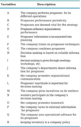
The population was made up by 93 industrial SMEs of Ibague according to its Chamber of Commerce’s registries. The sample of 76 organizations: 66 small and 10 medium-sized was selected through stratified simple random sampling with correction due to finite population. An error of 5% and reliability of 95% were assumed. As primary source of information a Likert scale-type questionnaire was employed, with the options always, almost always, sometimes, almost never, never and doesn’t know doesn’t respond, which are included the questions contained in Table 1 and were justified in the theoretical framework. With respect to the empirical contrast of the data collecting instrument, its reliability represented by Cronbach’s alpha coefficient for the whole questionnaire was 0.893; which according to the scale of Ruíz (2002) is very high and points to its internal consistency (Corbetta, 2007; Hernández et al., 2010; Jérez, 2001; Ghauri and Gronhaug, 2010). Likewise for the dimensions: planning and organization of the prognoses and the prognoses and direction, this coefficient was 0.894 and 0.617 respectively.
In order to achieve the final objective, a binary logistic regression model was developed in which the dependent variable was “the company performs prognoses for its different operations” (REALPRO) and as independent variables were taken the original attributes of the study listed in Table 1, separated among the dimensions: planning and organization of prognoses which included variables from “C” to “L”, and the prognoses and direction which comprised attributes from “M” to “R”.
4. Results and discussion
At first instance were taken the variables related to the “planning and organization of prognoses” dimension in order to stablish which of them had an incidence on the dependent variable “REALPRO”. In this sense, each one of the outcomes from SPSS-21 will be explained.
The codification of the dependent variable which in fact must be dichotomous, signalizes that a value of zero (0) was assigned to those SMEs that do perform prognoses and a value of one (1) to those who do not employ such tool. On the other hand, the model’s verosimilitude (-2L) shows the extent to which it fits the data well, and the smaller this value the better its fitting. In this scenario as only the constant was introduced, preliminary estimatives equal 55.293 for verisimilitude and 2.007 for the constant(b0).
Regarding the regression model’s classification, by comparing the forecasted values against those observed and taking as basis the (Y) dependent variable’s probability’s cutting value of (0.5), it classifies as REALPRO=YES meaning they do employ prognoses; whereas if such probability is > 0.5, they are deemed as REALPRO=NO, meaning that these organizations do not employ prognoses tools. In this first step, the model has classified 88.2% of the cases correctly and no company that “does not perform prognoses” has been classified correctly.
Next, Table 2 presents the estimated parameter (B), its standard error (ET) and its statistical meaning with the Wald test, which is a statistic that follows a Chi square with 1 degree of liberty (gl) and the estimation of the OR (Exp (B)). As can be seen in the equation of regression of step zero only the constant appears, having left out the other variables from the dimension of analysis. However, as may be appreciated on Table 3 all variables, except for attributes “I” and “K”, have a statistical significance of 0.00 associated to Wald’s index; which is why the process will continue in order to incorporate all or some of them into the equation.
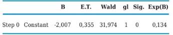

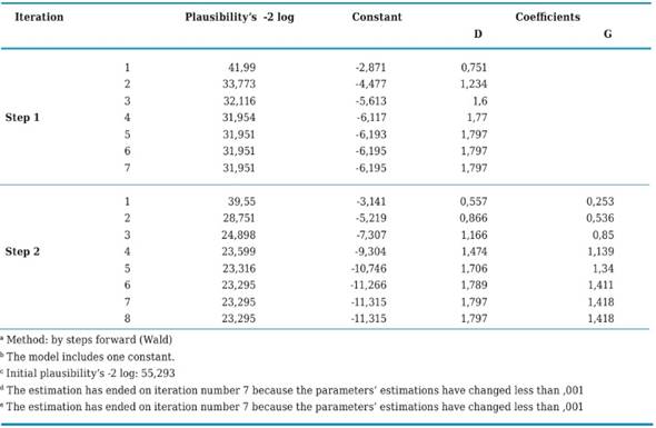
Table 4 displays the iteration process which now applies for three coefficients, the constant that had already been included in the previous step, and variables “D” (prognoses significantly influence organizational performance) and “G” (the company combines qualitative and quantitative prognoses for decision making). As may be observed in this case, statistic - 2LL decreased with respect to the previous step which only borne one constant and whose value was 55,293, whereas now it decreased to 23,295. This process ends with 8 loops and the calculated coefficients were: constant b0 = -11,315 and for the “D” and “G” variables b1 = 1,797 y b2 = 1,418 respectively.
Likewise, the Omnibus test which by means of Chi Square asses the null hypothesis that the coefficients of all terms included in the model except for the constant equal zero, casts for this case the difference between the value of -2LL for the model that only included the constant, and the value of -2LL for the current model as follows:
Chi squared = (-2LL model 0) - (-2LL model 1) = 55,293 - 23,295 = 31,998
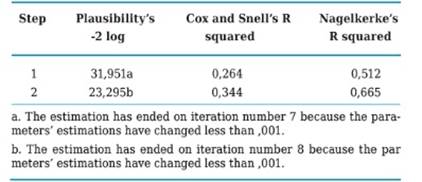
In this study’s particular case, it can be made evident that the model with the new two variables introduced “D” and “G” improves its fit with respect to its previous situation, which is corroborated by the 0,000 level of statistical significance. In the model’s summary presented in Table 5 appear two complimentary statistics to the plausibility ratio (RV), which are employed to evaluate its validity in a global manner, those being the coefficients of determination R2, Cox’s y Snell’s which explain the dependent variable’s variation (Y) based on the predicting attributes’ value changes (independent variables) that in this case are “D” and “G”. Here it may be seen that in step 2, plausibility decreased significantly as it had been previously mentioned and Cox’s and Snell’s and Nagelkerke’s coefficients report the two independent variables explaining the model at 34.4% and 66.5% respectively, which are deemed as sound estimates taking into account that only two out of the 10 original variables were considered.
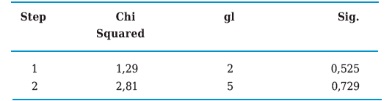
Homer and Lemeshow’s test is another statistic also used to assess the goodness of fit of a logistic regression model. It starts from the fact that if the fit is good, a high value of the estimated probability (p) will associate with the result “1” of the binomial dependent variable, whereas a low p value (close to zero) in most cases will correspond with the result Y=0. In this case, the level of significance was 0.729 in the second step, which demonstrates the model’s goodness of fit (Table 6).
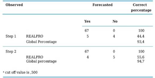
The classification chart to be presented next on shows this model as having a high specificity (100%), a relatively high sensitivity (55.6%) and a global percentage of 94.7% including the constant and the two independent variables (D and G), which indicates that the model is classifying relatively well those SMEs who do not perform prognoses (Table 7). At the same time, Table 8 shows the variables that went into the model, its regression coefficients with their respective standard error, Wald’s statistical value used to assess the null hypothesis (βi = 0), the statistical significance associated and the value of OR (Exp (B)) with its confidence intervals.
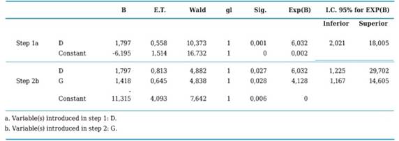
With the data contained in Table 8, it’s possible to build the logistic regression equation (Formula 1), which would look as follows:
This algorithm is useful to predict the probability of obtaining the “NO” result (REALPRO); a company which does not apply prognoses techniques with regards to “D” (prognoses significantly influence organizational design) and “G” (the company combines qualitative and quantitative prognoses in decision making). This way, according to the logistic equation (Formula 2 and Formula 2.1), an organization with (D=1) and G (1) would have a probability of not carrying out prognoses equal to:
With this probability’s result, which is less than 0.50 as it may be observes, it is possible to state that based on the variables Ibague’s industrial SMEs “prognoses significantly influence organizational performance” (D) and “the company combines qualitative and quantitative prognoses in decisions making) (G), have a significant probability of applying prognoses techniques to their operations.
This finding permits to corroborate the importance that Ibague’s industrial SMEs businessmen bestow on prognoses as vital tools for their organization’s development, which confirms the approaches by Russell and Taylor (1995), Reid and Sanders (2010), Schroeder et al., 2011, Krajewski et al., (2010), Heizer and Render (2011) y Meredith & Shafer (2010) regarding the influence that prediction techniques have on decisions related to production planning and programming, financial planning, and highest-end strategic planning.
On the other hand, combining different prognoses tools constitutes a key aspect when deciding whether or not to apply forecasting techniques within Ibague’s industrial SMEs, which coincides with the arguments of Makridakis et al. (1978) when emphasizing the importance of combined prognoses methods on the exactitude of forecasts (Winkler and Makridakis 1983; Fildes, 1989; Bunn and Vassilopoulus, 1999).
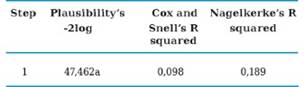
In second term were taken variables related to the “prognoses and direction” dimension in order to stablish of them had an influence on the dependent variable “REALPRO”. Table 9 shows the iterations history for this new model, which compares original iterations finding that it now applies to two coefficients; the constant included in the previous step (Table 2) to two coefficients; the constant included in the previous step (Table 2) and the “P” variable (prognoses significantly influence organizational performance). This case shows that the -2LL statistic decreased with respect to the previous step which only borne the constant and whose value was 55,293, while now it was reduced to 47,462. This process finalizes with 6 loops and the calculated coefficients were: constant b0 = - 4,205 and for the variable part “P”, b1 = 0,660.

The Omnibus test presented on Table 10 shows the Chi squared for the model that only included the constant and -2LL’s value for the current model, which comprised both the constant and the “P” variable.
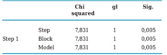
Chi squared = (-2LL model 0) - (-2LL model 1) = 55,293 - 47,462 = 7,831
As it may be seen, by introducing the new “P” variable the model improves its fit with regard to its previous situation, which is corroborated by the 0,005 level of statistical significance.
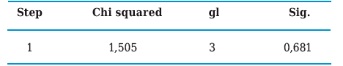
Table 11, corresponding to the model’s synthesis, shows that the plausibility ratio decreased a little, whereas the R2 and Cox’s and Snell’s determination coefficient point to the independent variable explaining the model at 9.8% and 18.9% respectively; even though they’re low, they are deemed acceptable since only one variable was taken into account out of the second dimension’s 6 original variables. Hosmer and Lemeshow’s test in this case displayed and significance rate of 0,681, which shows the model’s goodness of fit (Table 12).
A new classification of the model shows it to have high specificity (100%) and null sensitivity (0%). With the constant and the only independent variable included (P) in the model, it classifies SMEs who do not perform prognoses poorly when Y’s probability’s cut off point is stablished at 50% (0.5) by default. Likewise, Table 13 displays the variable that entered the model, its regression coefficient with its corresponding standard error, Wald’s statistical value used to calculate the null hypothesis (βi = 0), its associated statistical significance and OR’s value (βi = 0) with its confidence interval.

The building of the logistic regression equation (Formula 3) proceeds with table 13 information and it would be as follows:
This algorithm is useful in order to predict the probability of having the “NO” result (REALPRO), a company who does not apply prognoses techniques with regard to “P” (the company turns to external information to perform its prognoses). As such, an organization with (P=1) would have, according to the logistic equation (Formula 4 and Formula 4.1), a probability of not performing diagnoses equal to:
Based on formula 4.1’s result, which is lower than 0.50, it’s possible to state that Ibague’s industrial SMEs, based on the variable “the company turns to external information to perform its prognoses” (P), have a significant probability of applying projection techniques to their operations. Within this context Genç et al., (2012), Stone and Fiorito (1986), Finney (2012), Oliva and Watson (2012), Raspin and Terjesen (2007), Hogarth and Makridakis (1981), Daniells (1981), Herbig et al., (1993), highlight external information’s importance as a vital input in order to apply prognoses techniques.
5. Conclusions
Prognoses constitute a vital tool within the process of decision making of different organizations. There’s not a single organizational area where the usage of these techniques isn’t required for the rationalization of resources. Within this context, the study referred in this article permitted to establish that a forecasting system bears a multidimensional character; that is to say, it cannot be seen from particular perspectives, on the contrary it required a holistic vision, which was made evident in the analysis of 18 variables that were considered, which, some to a higher extent than others, exercise some kind of influence when applying prognoses in these organizations. From this perspective, these businessmen acknowledge the importance borne by concepts such as planning, organizational structure, communication and information systems, training processes, incentives, teamwork, software, management of inventories and decision making in implementing these forecasting instruments.
Through the multivariate analysis logistic regression model, it was possible to corroborate that out of all the attributes considered those exercising the most influence on Ibague’s SMEs’ businessmen to apply prognoses in their companies are: “prognoses significantly influence organizational performance” and “the company combines quantitative and qualitative prognoses in decision making” from the planning and organization of prognoses and “the company turns to external information to perform its prognoses” from the prognoses and direction dimension

