DOI: http://dx.doi.org/10.15446/ing.investig.v35n3.50552.

Enhanced method for flaws depth estimation in CFRP slabs from FDTC thermal contrast sequences

Método mejorado de estimación de profundidad de defectos en láminas de CFRP a partir de secuencias de contraste térmico CTDF

A.D. Restrepo-Girón¹

¹ Andrés David Restrepo Girón: Electronic Engineer, M.Sc. in Automation, Ph.D. in Engineering, Universidad del Valle, Colombia. Affiliation: School of Electrical and Electronic Engineering, Universidad del Valle, Colombia.
E-mail: andres.david.restrepo@correounivalle.edu.co.

How to cite: Restrepo-Girón, A.D. (2015). Enhanced method for flaws depth estimation in CFRP slabs from FDTC thermal contrast sequences. Ingeniería e Investigación, 35(3), 61-68. DOI: http://dx.doi.org/10.15446/ing.investig.v35n3.50552.

ABSTRACT

After the detection of internal defects in materials, the characterization of these plays a decisive role in order to establish the severity of these flaws. Finite difference thermal contrast (FDTC) is a new technique proposed recently for contrast enhancement in sequences of thermal images in order to allow the detection of internal flaws in composite slabs with greater probability of success. Besides FDTC, a criterion was also conceived for the estimation of the depth of the detected defects, which brings good results for shallow and strong contrast defects, but poor estimations for deeper and weaker defects. Considering this problem, a revision of the original criterion is carried out in this paper to define a new and robust criterion for estimating the depth of defects, applied after FDTC enhancement and flaws detection. Results of the execution of the revised algorithm on a synthetized thermal sequence from an artificial CFRP slab (using ThermoCalc6L software) show a better performance of the estimation task, reducing the average relative error by more than half.

Keywords: Pulsed thermography, composite materials, thermal contrast, FDTC.

RESUMEN

Posterior a la detección de defectos internos en los materiales, su caracterización juega un papel decisivo para establecer la severidad de dichas fallas. El contraste térmico por diferencias finitas (CTDF) es una técnica novedosa propuesta recientemente para el mejoramiento del contraste en secuencias de imágenes térmicas que permite la detección de fallas internas en láminas de material compuesto con mayores probabilidades de éxito. A la par con el CTDF, se concibió un criterio de estimación de la profundidad de estos defectos que, aunque brinda buenos resultados para aquellos superficiales y más contrastados térmicamente, pierde calidad en la estimación de la profundidad de defectos más profundos y más débiles en su contraste térmico. Considerando este problema, en este artículo se adelanta una revisión de dicho criterio con el ánimo de definir un método más robusto para el cálculo de profundidad de los defectos contrastados por la técnica CTDF. Los resultados de la ejecución de este nuevo algoritmo sobre imágenes sintéticas generadas a partir de una lámina artificial de CFRP (mediante el software ThermoCalc6L) muestran un mejor desempeño en la estimación, reduciendo el error relativo promedio a más de la mitad.

Palabras clave: Termografía pulsada, materiales compuestos, contraste térmico, CTDF.

Received: May 8th 2015 Accepted: August 20th 2015

Introduction

Nowadays, composite materials like Carbon Fiber Reinforced Plastic (CFRP) play a crucial role for aeronautical and automotive industry due mainly to the better strength/ weight relation with respect to common metallic materials. Nevertheless, the increased use of composites makes it necessary to implement suitable inspection techniques to ensure their quality and reliability (IATA, 2009; Pohl, 1998). For this purpose, Pulsed Thermography (PT) is a non­destructive evaluation (NDE) technique that has become a mature and important procedure in the task of analyzing composite materials, given its non-invasive and non-contact features (Bagavathiappan, Lahiri, Saravanan, Philip & Jayakumar, 2013). In an experiment of PT, a flash is used to heat the material under inspection and a sequence of infrared (IR) images or thermograms are recorded by a thermal camera; later, cooling profiles at every pixel are extracted from these images to be processed and make possible the detection and characterization of internal defects or flaws (Benítez, Loaiza & Caicedo, 2011). However, flashing a surface makes the heating pulse spatially non-uniform (Ibarra-Castanedo, 2005), and so, the background thermal behavior influences adversely the subsequent detection and characterization stages. To overcome this problem, a thermal contrast enhancement (directly related to IR image contrast) needs to be carried out.

Many different processing methods are proposed to deal with this challenge, making use of time resolved techniques (Larsen, 2011), polynomial fitting of thermal profiles (Balageas, Roche, Leroy, Liu & Gorbach, 2015), mathematical transforms (Marinetti et al., 2004; Rodríguez, Ibarra-Castanedo, Nicolau & Maldague, 2014a), frequency space conversion (Ibarra-Castanedo, 2005), or heat propagation models (Rodríguez, Nicolau, Ibarra-Castanedo, & Maldague, 2014b). Generally, the more accurate models take into account the three spatial dimensions and, at the same time, intend to reconstruct the temperature distribution at each time instant through a grid of points covering the surfaces and the inside body of the inspected material (Grinzato, Bison, Marinetti & Vavilov, 2000; Cheng-Hung & Meng-Ting, 2008; López, Nicolau, Ibarra-Castanedo & Maldague, 2014); this fact makes these models complex and heavy.

Accordingly, Finite Difference Thermal Contrast (FDTC) method was proposed to work with a discretized and reduced 3D heat propagation model to give a relative thermal estimation error, leading to a normalization procedure that brings stronger contrast profiles and, consequently, greater probability of detecting deeper defects without requiring an a priori selection of a sound area or a reference image (Restrepo & Loaiza, 2014a). For each pixel in each thermogram, and at every time instant, FDTC only estimates the value of temperature in the next time on the frontal surface of the specimen, based on actual temperature data of the same pixel and its neighbors. This feature not only makes this technique faster, but also more reliable. Additionally, this technique takes advantage of another contrast enhancement method proposed by the FDTC authors named Background Thermal Compensation by Filtering (Restrepo & Loaiza, 2013; Restrepo-Girón & Loaiza, 2014b) to flatten sound profiles even more and make defective profiles tend to zero with time.

FDTC uses the approximation to the time solution of the classic 3D heat propagation differential equation, introduced earlier by Tadeu and Simoes (2006) for several configurations of diffusion mediums and different propagation ways. Specifically, the approximation defined for a slab medium is used in defects detection purposes, and the solution for a semi-infinite medium is used in defects depth estimation, for which a limited and simple method proposed in (Restrepo & Loaiza, 2012) was implemented. In this work, this depth estimation method is revised in order to achieve smaller errors. For this purpose, in the next section a brief summary of FDTC mathematical models and the foundations of the depth estimation technique are presented. Later, the modifications proposed will be discussed, followed by comparative results between the revised and original estimation methods applied to an artificial IR sequence. Finally, conclusions will show the relevant facts about the revision carried out.

FDTC method for detection and depth char­acterization of internal defects

Contrast enhancement

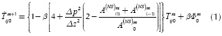
The FDTC procedure is supported in the slab 3D differential thermal estimation model (Restrepo & Loaiza, 2012):

Where

• 

• 

• 

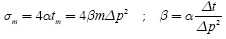
• Δx=Δy=Δz=spatial differential step;

• h = slab thickness.

• NS = arbitrary number of times that the heat wave reflects on both surfaces inside the slab, according to actual model.

• t_m = m.Δt, with m = 0,1,2,...,M-1, being M the total number of thermograms acquired, and Δt the acquisition period of the images;

• x_i = i.Δx, with i = 0,1,2,..., N_x-1, being N_x the total number of rows in each image;

• y_j = j.Δy , with j = 0,1,2,..., N_y-1, being N_y the total number of columns in each image;

• z_k = K.Δz , with k = 0,1,2,..., Nk-1, being N_k the total number of steps dividing the thickness of the slab. The value of Nk is unknown in a real PT experiment;

• α = being the thermal diffusivity of the specimen.

• T^m_ij0 being temperature on pixel i, j, k for thermogram m.All images correspond to temperature distribution over the specimen surface, so k = 0

The expression in Equation (1) comes from an initial discretization by finite differences in an explicit way of the complete 3D model of heat propagation through a specific medium. Considering that the specimen is isotropic and homogenous, the thermal excitation is very similar to an impulse function. No heat is generated inside the slab, and there are no losses by convection through its surfaces (i.e., after thermal excitation, heat flux is only due to conduction phenomena inside the slab, which makes heat spread throughout the slab until thermal equilibrium is reached).

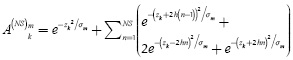
Since the discrete terms modeling the contribution in heat flux along the depth axis (z axis) are not directly measurable from surface temperature images, it was assumed that lateral heat dispersion was negligible for a thermal propagation of Az, and so, they were replaced by the expressions obtained from approximated solutions of the differential equation of heat diffusion applying Green Functions, proposed by Tadeu and Simões (2006).

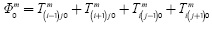
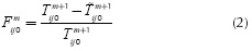
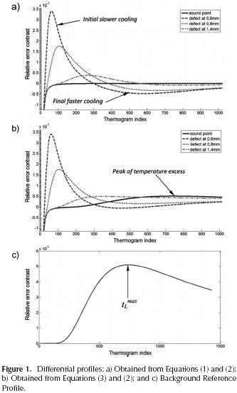
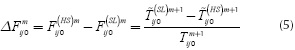
Finally, applying this equation, the next value of temperature (in the time domain) for each pixel is predicted. If T^m+1and ^m+1_ijO denote, respectively, the real and the estimated next temperature for a specific pixel, F^m_ij0 in Equation (2) represents the relative error in estimation, which may be expected to be less for pixels corresponding to healthy zones than for pixels laying on defective areas; this feature leads to enhanced contrast images. Then, taking F^m_ij0 along time (m = 0, 1, 2,..., M-1)we have differential error profiles which will be different between defective and healthy points, as shown in Figure 1a.

The previous method constitutes the basis of the FDTC technique. The most relevant fact in applying it is that the decay rate of FDTC profiles for defect points, when the flaw depth increases, is less than the decay rate evidenced in other time-resolved techniques, which becomes a factor for better global contrast and, as a consequence, results in a greater probability of defects detection with a smaller diameter/depth ratio (Restrepo & Loaiza, 2014a).

Depth estimation

In an IR thermography experiment, once internal defects are found, it is desirable to estimate the depth at which each one was found, among other features. If we use the solution corresponding to a semi-infinite propagation medium, assuming null normal flux at the surface (once irradiated heat increases the frontal surface temperature, the model assumes that there is no heat flux returning from the surface to the surrounding medium), we have the Half­space 3D Differential Thermal Estimation:

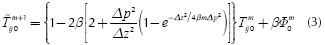
Figure 1b reveals examples of differential profiles obtained with FDTC based on both Equation (3) and the relative error of Equation (2). What is interesting here is that previous profiles (even those for sound points of material) do not tend to zero as in Figure 1a, but exhibit a positive peak of temperature excess, as if healthy regions of material were cooling slower than expected. This phenomenon is related to the presence of the back surface of the slab that reflects the thermal wave, since this reflection would not exist if the medium were semi-infinite.

From this point, and assuming very thin flaws with a large diffusivity compared to that of the slab material (as the situation where there are delaminations inside composite slabs), a basic mathematical criterion to estimate the depth of detected flaws is used:

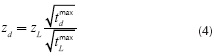
Where:

• t^max_d is the peak time instant of the differential profile corresponding to a specific defect obtained from FDTC based on Equation (1);
• t^max_T is the peak time instant of any differential profile corresponding to a healthy point obtained from FDTC based on Equation (3);
• z_d is the depth to estimate;
• z_L is the thickness of the slab.

For its part, the particular form of the healthy profile in Figure 1b is reproducible in a very similar way if any profile yielded by FDTC based on Equation (1) is subtracted from the corresponding profile (the same i and j parameters) yielded by FDTC based on Equation (3) as presented in Figure 1c (Restrepo-Girón & Loaiza, 2015). Furthermore, this resulting profile is practically the same whatever the selected pair of corresponding profiles and, for that reason, it will be identified from now as Background Reference Profile. Consequently, t_L^max could be taken as the peak time instant of this reference profile.

Revision of depth estimation method

Despite the advantage of generating a background reference profile from subtraction of corresponding differential profiles obtained with both previous discretized models for FDTC, there are two aspects that may adversely influence an estimation task: a) noise in real sequences can make peak time instant vary slightly according to the pair of corresponding profiles selected to be subtracted to generate the background reference profile; b) additionally, since t_d^max belongs to a differential profile obtained from FDTC based on Equation (1), where healthy profiles do not exhibit a similar behaviour than background reference profile, but tend to zero during almost all of the time axis, the peak time instants suffer a left shift in time, more appreciable for profiles taken from deeper defects.

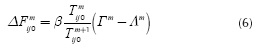
Regarding the first issue, the background reference profile can be produced in a more analytical way, subtracting the previous models from which differential profiles are generated. If we call F(^SL)^m_ijO and F(^HS)^m_ijO the relative errors, given the pixel(i,j) at the thermogram m, for FDTC method using the slab approximation and the half-space approximation, respectively, the model of the background reference profile would be equivalent to:

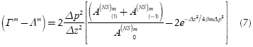
Taking Equations (1) and (3) and denoting:

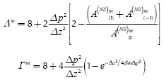
we have:

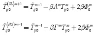
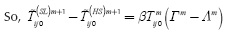and finally

Where:

According to Equation (6), one profile is needed to extract the temperature values T™_ij0 and T^m+1_ij0 at each iteration of the algorithm. However, knowing that the background reference profile is practically the same whatever the selected pair of corresponding proiles, if we choose a healthy proile we will be sure that temperature values do not change considerably along time, and therefore, we can assume that: T^m+i_ijO ≈ T^m_ijO . In this way, Equation (6) can be reformulated

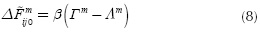
Taking all valid values for m, Equation (8) introduces an analytical model for the background reference profile shown in Figure 1c, making it unique for a specified sequence and allowing it does not require any selection of thermal profiles. So, returning to Equation (4), the parameter t_L^max would then be the peak time instant of this analytical profile.

Regarding the second issue mentioned above, and analyzing the performance of Equation (4), it can be concluded that t^max_d instants tend to be smaller than they should be for acceptable estimation of deeper defects (Restrepo-Girón & Loaiza, 2015). The reason for these results is the fact that using the FDTC version based on Equation (1) to evaluate t_d^max parameters, we have to work with defective profiles that do not exhibit the implicit presence of elevation contrast produced by the opposite face of the slab. Therefore, we would initially think of using the FDTC version based on Equation (3) to take all of the t_d^max parameters as a suitable solution; but in this case, unfortunately, differential profiles corresponding to the deepest defects become distorted enough to get too close to the reference peak (at t_L^max).

To deal with this problem, we suggest the use of defective differential profiles obtained from FDTC version based on Equation (1), which will be called ; but this time we will add the background reference profile, denoted by ,to every one of them to obtain distorted profiles defined as . Also, let us define:

• max(), max (), max (): global maximums of , and .
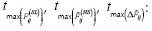• pead time instants of , and

When the previous addition is carried out, the next possible results can be observed, as depicted in Figure 2.

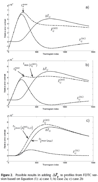
1. max is greater than max () as in Figure 2a. In such case: ..
2. max ()is equal to or smaller than max () in which case a local minimum is searched among () and t _{max( )}. Assuming the minimum to be located at t , this result derives into two possibilities:
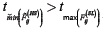1. which means that a second peak (local maximum) can be found in the interval 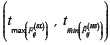as in Figure 2b. So, if is the time instant of this new peak, we have: .
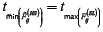2. which means that the only peak in the searching range is at ; but this time tends to be too close to when is weaker than distorting estimation results. In this case, the next procedure is proposed:
1. Find the left half value of max( )and its corresponding time instant: .
2. Find the left half value of max()and its corresponding time instant:
3. Apply Equation (4) using time instants at half values of corresponding peaks (see Figure 2c):

Synthesis of the analytical background reference profile and execution of the previous algorithm makes it possible to enhance the performance of the estimation criterion represented in Equation (4), as the next section will describe.

Results analysis of the modified FDTC depth estimation method

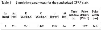
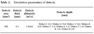
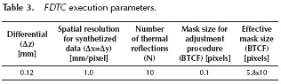
To assess the performance of the modified FDTC depth estimation, without the influence of noise, emissivity or any optical distortion, a sequence of IR images obtained from a simulated squared CFRP slab, 2 mm thick, with 9 air-filled defects (Figure 3) was used. This sequence was synthetized by using ThermoCalc6L software with parameters listed in Tables 1 and 2, assuming the flashing focus on the center of images. For thermal enhancement purposes, FDTC was applied to the sequence with parameters registered in Table 3.

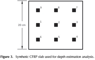
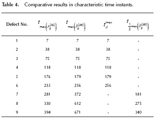
In order to evaluate the revised method, the differential profile corresponding to the centroid of each defect in Figure 3 was taken as , and the background reference profile was generated by the application of Equation (8). The discrete time instants at the maximum of and its left half value were respectively 740 and 388, which are equivalent to 4.66 and 2.44 seconds for this sequence. All of the differential profiles were smoothed by an iterative 3^rd order Savitzky-Golay filter. Tables 4 and 5 show characteristic discrete time instants (thermogram indexes) for differential profiles, and the estimated depth for each defect using the original criterion and the revised criterion as well. For its part, Figure 4 displays the linearity of both versions of the method.

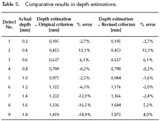
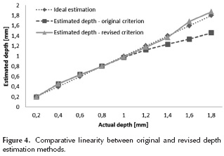
The more relevant thing that can be seen is the notorious deviation of depth estimation from the ideal performance for depths greater than half of the slab thickness, when strictly using the reason between peak time instants of profiles and . When using the revised method the problem is corrected, leading to a better behavior of the relative error for those deeper defects. In fact, the average absolute relative error is reduced from 8.7 % to 4.2 %, and the worst absolute error for deeper defects decreases from 18.9 % to 5.2 %. The performance at shallow defects remains unaffected, as it was expected; but the estimation of depth for the 0.4 mm defect has an atypical deviation caused by some artifact introduced by the contrast enhancement technique or the previous noise filtering procedure.

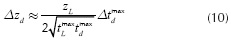
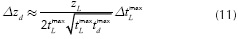
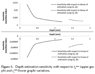
If we take partial derivatives of Equation (4) with respect to peak time instants to define sensitivity coefficients, the variation of z_d for small variations of t_d^max and t_L^max can be approximated respectively by Equations (10) and (11). Figure 5 shows the approximated behavior of these sensitivities.

Identical expressions are obtained in cases where and must be used. It is clear that, in general, the closer that defects are from the irradiated surface, the more sensitive the depth estimation to the uncertainty of calculated t_d^max and t_L^max. This fact helps to explain why the greater error in Table 5 belongs to the defect at 0.4 mm depth. Nevertheless, shallower defects usually have a greater SNR, which makes them easier to characterize. However, it is interesting that in using and the sensitivity magnitude rises again, though it resumes the same decreasing behavior with respect to depth. For its part, depth estimation is much less sensitive to variations of t_L^max, which will be ever greater than the other characteristic time instants.

Conclusions

In this paper a simple criterion to estimate the depth of defects detected inside slabs, after processing the sequences of thermal images with Finite Difference Thermal Contrast (FDTC), is revised and modified in order to enhance its performance. The original depth estimation criterion works with an approximated solution to the discretized heat propagation model for semi-infinite mediums; because FDTC contrast profiles result from heat propagation inside a slab medium, the use of the semi-infinite medium model creates a late deformation on differential contrast profiles caused by the presence of the opposite face of the slab, not considered in this model.

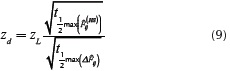
The deformation described plays the role of time reference to calculate the depth of detected defects, previously knowing the slab thickness. But for deeper defects, working with peak time instants of differential profiles obtained from Equation (1) or from Equation (3) exclusively, large errors can arise. So, the revision of the method led, in general, to two modifications: first, an analytical background reference profile is synthetized from a suitable mix of the two discretized models used before for FDTC according to Equation (8), bringing a reference of the opposite face of the slab, independent from any pixel selection. Second, an algorithm that adjusts the characteristic time t_d^max of Equation (4), depending on intensities of differential profiles with respect to that of , and even, modifies slightly Equation (4) into Equation (9) when using the instants at left half-values of peaks is more reliable for the estimation task. Executing this modified criterion an average error of 4.2 % and a maximum error of 5.2 % for deeper defects were achieved, in comparison to the errors of 8.7 % and 18.9 %, respectively, resulting from the original version. For future work, the revised estimation criterion must be carried out in real sequences of thermal images where noise, distortions and other artifacts alter pixel intensities, to establish the practical robustness of this method.

References

Bagavathiappan, S., Lahiri, B., Saravanan, T., Philip, J., & Jayakumar, T. (2013). Infrared thermography for condition monitoring - A review. Infrared Physics & Technology, 60, 35-55. DOI: 10.1016/j.infrared.2013.03.006.         [ Links ]

Balageas, D., Roche, J., Leroy, F., Liu, W., & Gorbach, A. (2015). The thermographic signal reconstruction method: A powerful tool for the enhancement of transient thermographic images. Biocybernetics and Biomedical Engineering, 35(1), 1-9. DOI: 10.1016/j.bbe.2014.07.002.         [ Links ]

Benítez, H., Loaiza, H., & Caicedo, E. (2011). Termografía activa pulsada en inspección de materiales. Técnicas avanzadas de procesado. Cali, Colombia: Universidad del Valle—Pontificia Universidad Javeriana.         [ Links ]

Cheng-Hung, H., & Meng-Ting, C. (2008). A transient three-dimensional inverse geometry problem in estimating the space and time dependent irregular boundary shapes. International Journal of Heat and Mass Transfer, 51, 5238­5246. DOI: 10.1016/j.ijheatmasstransfer.2008.03.019.         [ Links ]

Grinzato, E., Bison, P., Marinetti, S., & Vavilov, V. (2000). Thermal NDE enhanced by 3D numerical modeling applied to works of art. Paper presented at 15th World Conference on Non-destructive Testing, Rome, Italy. Retrieved from http://www.ndt.net/article/wcndt00/papers/idn909/idn909.htm.         [ Links ]

International Air Transport Association. (2009). A Global Approach to Reducing Aviation Emissions. First Stop: Carbon-Neutral Growth from 2020.Switzerland: International Air Transport Association.         [ Links ]

Ibarra-Castanedo, C. (2005). Quantitative Subsurface Defect Evaluation by Pulsed Phase Thermography: Depth Retrieval with the Phase (Doctoral dissertation). Available from Collection Mémoires et thèses électroniques, Université Laval.         [ Links ]

Larsen, C. (2011). Document flash thermography (Master of Science Thesis). Available from Utah State University DigitalCommons@USU.         [ Links ]

López, F., Nicolau, V., Ibarra-Castanedo, C., & Maldague, X. (2014). Thermal-numerical model and computational simulation of pulsed thermography inspection of carbon fiber reinforced composites. International Journal of Thermal Sciences, 86, 325 - 340. DOI: 10.1016/j.ijthermalsci.2014.07.015.         [ Links ]

Marinetti, S., Grinzato, E., Bison, P.G., Bozzi, E., Chimenti, M., Pieri, G., & Salvetti, O. (2004). Statistical analysis of IR thermographic sequences by PCA. Infrared Physics & Technology, 46, 85-91. DOI: 10.1016/j.infrared.2004.03.012.         [ Links ]

Pohl, J. (1998). Ultrasonic inspection of adaptive CFRP-structures. Paper presented at the 7th European Conference on Non-Destructive Testing (ECNDT), Copenhagen, Denmark. Retrieved from http://www.ndt.net/article/ecndt98/aero/015/015.htm.         [ Links ]

Restrepo, A., & Loaiza, H. (2012) New method for basic detection and characterization of flaws in composite slabs through Finite Difference Thermal Contrast (FDTC). Paper presented at the 11th International Conference on Quantitative Infrared Thermography (QIRT), Image & Data Processing Session, Naples, University of Naples. Retrieved from http://www.ndt.net/article/qirt2012/papers/QIRT-2012-156.pdf.         [ Links ]

Restrepo, A., & Loaiza, H. (2013). Non-uniform heating compensation on thermal images using median filtering. DYNA, 80(182), 74-82.         [ Links ]

Restrepo, A., & Loaiza, H. (2014a). New 3d inite difference method for thermal contrast enhancement in slabs pulsed thermography inspection. Journal of Non-destructive Evaluation, 33(1), 62-73.         [ Links ]

Restrepo-Girón, A., & Loaiza, H. (2014b). Background thermal compensation by filtering (BTCF) for infrared thermography evaluation. In Proceedings of the XIX International Simposium of Signal and Images Processing and Artificial Vision (STSIVA, 2014). lEEEXplore. DOI: 10.1016/j.ndteint.2014.06.003.         [ Links ]

Restrepo-Girón, A., & Loaiza, H. (2015). 3D discrete model for thermal contrast enhancement and defects depth estimation in CFRP slabs. Ingeniería y Competitividad, 16(2), 143-153.         [ Links ]

Rodríguez, F. L., Ibarra-Castanedo, C., Nicolau, V., & Maldague, X. (2014a). Optimization of pulsed thermography inspection by partial least-squares regression. NDT & E International, 66, 128-138.         [ Links ]

Rodríguez, F. L., Nicolau, V., Ibarra-Castanedo, C., & Maldague, X. (2014b). Pulsed Thermography Signal Processing Techniques Based on the 1D Solution of the Heat Equation Applied to the Inspection of Laminated Composites. Materials Evaluation, 72(1), 91-102.         [ Links ]

Tadeu, A., & Simöes, N. (2006).Three-dimensional fundamental solutions for transient heat transfer by conduction in an unbounded medium, half-space, slab and layered media. Engineering Analysis with Boundary Elements, 30, 338­349. DOI: 10.1016/j.enganabound.2006.01.011.         [ Links ]