


 Inglés (pdf)
 Articulo en XML
 Referencias del artículo
 Enviar articulo por email
 Citado por SciELO
  Citado por Google
  Similares en
SciELO
Similares en
SciELO  Similares en Google
 Permalink
Introduction
In recent decades, scientists around the world have been increasingly interested in studying soil organic carbon (SOC) and its relationship with climate change. A potential impact of global warming is the accelerated decomposition of SOC and an increase in the carbon released into the atmosphere (Jia et al., 2017). Rising levels of CO2 concentration in the atmosphere have led a considerable part of the scientific community to contemplate SOC sequestration as an alternative to mitigate climate change, which can be achieved through various management practices based on increasing the SOC stock (SOCS) (Huang et al., 2019).
Through photosynthesis, plants are able to capture carbon from the atmosphere and integrate it into their own structure (biomass), as well as into the soil through their radicular systems. This phenomenon can also be called carbon sequestration (Stockmann et al., 2013) and has a special focus on agricultural land due to the fact that around 37% of the planet's surface is destined for agricultural use (Sommer and Bossio, 2014).
In order to monitor the SOCS, it is necessary to acquire information on the soil bulk density (BD) and the SOC and subsequently analyze the changes in these variables over different periods of time according to the established needs. However, the resources needed to conduct these kinds of studies are expensive and time-consuming because of the standard laboratory analyses and procedures involved (Camacho-Tamayo et al., 2014; Liu et al., 2019). Soils are also characterized by being a heterogeneous material in both spatial and temporal scales, often causing SOCS studies to require a high sampling density (Cambou et al., 2016). Therefore, it is necessary to explore SOCS analysis techniques that represent a reduction in the resources required.
Chemometric approaches constitute a potential tool to evaluate soil attributes rapidly and accurately in the laboratory (Ben Dor et al., 2015; Davari et al., 2021 ). Diffuse reflectance spectroscopy is a technique developed to accelerate data acquisition regarding materials' properties. Soil spectroscopy is based on the idea that the characteristics of the radiation reflected by a material when exposed to an electromagnetic spectrum depend on the composition of the material itself. This means that studying soil reflectance can provide information about the properties and condition of the soil under study (Davari et al., 2021; Viscarra Rossel and Webster, 2012). The features of the reflected spectra of a soil sample in the NIR spectrum have allowed for optimal results in terms of predicting soil properties, especially when dealing with SOC assessments (Liu et al., 2019; Nawar and Mouazen, 2019; Nocita et al., 2014).
It is important to mention that the acquisition of spectral signatures can be carried out in situ or using laboratory equipment. This can affect the information obtained from the reflectance spectra, causing variations in the model performance with regard to the estimated properties (Ahmadi et al., 2021; Ben Dor et al., 2015). When spectral signatures are taken in situ, factors such as the contact probe device of the equipment and its operator, the moisture of the soil sample, and environmental conditions can alter the spectral reflectance of the samples in comparison with those acquired in the laboratory. The latter would then be assumed to have been acquired under controlled environmental conditions, as well as after being dried and sieved for the sake of homogeneity.
The objective of this research was to evaluate the potential of NIR spectroscopy in order to estimate the SOCS of oxisols in the study area. Several models were developed by varying the number of samples used for calibration, followed by the evaluation of the spatial variability of the measured and estimated data by means of depth splines and geostatistical interpolated surfaces.
Materials and methods
Study area and field sampling
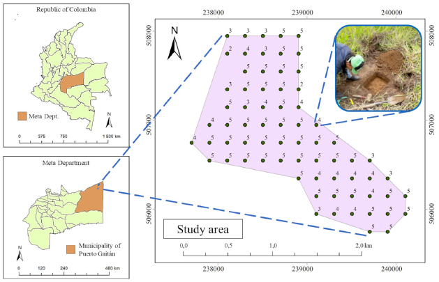
This study was carried out at the Carimagua Experimental Station of Agrosavia, located in the municipality of Puerto Gaitán (Meta, Colombia), with geographic coordinates 4° 34' 48" N, 71° 21' 00" W, an average altitude of 175 masl, an average annual temperature of 28 °C, an average rainfall of 2 240 mm, and a warm-humid climate. The relief of the study area is flat to slightly undulating, with slopes ranging between 0 and 7%. Soils are mostly oxisols whose dominant taxonomic component is typic hapludox. These soils have a low pH (<5), are well drained, and are covered with native savanna. Their predominant use is extensive livestock farming.
The study area has an extension of 248 ha, where a directed sampling scheme was established. Sampling took place in 2018 and consisted of 70 points spaced perpendicularly by 200 m, from which soil samples were extracted in depth intervals of 0-10, 10-20, 20-30, 30-40, and 40-50 cm, for a total of five samples per trunk (Figure 1). The total number of samples collected was 313, out of which 70 corresponded to the first and second depths, 68 to the third, 59 to the fourth, and 46 to the last. The difference in samples collected per depth is attributed to the presence of the water table in the study area. Each of the 313 soil samples consisted of a disturbed sample and an undisturbed cylinder sample.
Laboratory analysis
The disturbed samples were dried at 35 °C and then sifted through a 2 mm mesh. Total soil carbon was determined using an elemental analyzer (TruSpec CN Carbon Nitrogen Determinator, LECO Corp., St. Joseph, MI, USA). Since the soil samples did not show the presence of carbonates in the hydrochloric acid test, the total carbon was considered to be the SOC. The undisturbed soil sample cylinders were oven-dried at 105 °C for 48 h, and then the BD was calculated by dividing the mass of the soil by the volume of the cylinder. The SOCS was determined according to Equation (1):
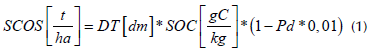
where DT stands for the depth and thickness of the soil layer, and Pd stands for the stoniness factor. In this case, Pd was assumed to be 0 because no significant stoniness was evidenced in the sampling process. Spectral signatures were recorded using a NIRFlex N-500 spectrometer (BÜCHI Labortechnik AG), which recorded measurements in reflectance units in the NIR range, from 1 000 nm to 2 500 nm, averaging 32 scans for each wavelength. The spectral signatures were taken from the dried and sieved soil samples.
Spectral modeling
To perform spectral modeling, it was first necessary to define the calibration and validation groups of the spectral models. The Kennard-Stone algorithm (Kennard and Stone, 1969) made it possible to establish uniformly distributed groups according to the variance of the spectral signatures. The calibration groups for BD and SOC were defined with 70% of the total signatures, while the validation group was assigned the remaining 30%. For SCOS spectral modeling, calibration groups consisting of 10, 20, 30, 60, 90, 120, 150, 180, 210, 240, and 270 samples were built with the Kennard-Stone algorithm. A subsequent validation of each group was carried out with the samples that did not take part in the calibration model.
In the model calibrations, spectral data were submitted to a series of pretreatments to normalize the responses and smooth out any possible noise that could be present in the signatures. The pretreatments considered were the transformation of raw spectra to absorbance, the Savitsky-Golay derivate, and standard normal variation. Once the combinations of pretreatments were applied, the model was built by means of PLSR, which is a commonly used technique when dealing with high-dimensional data (such as the wavelengths of the NIR spectral range) with highly collinear predictor variables. This technique summarizes the data into a few orthogonal factors, which are linear combinations of the predictor variables, so that the covariance of both the predictor and dependent variables is maximized. These orthogonal factors are then employed to develop a linear model to estimate the soil's attribute of interest (Katuwal et al., 2020).
The criteria to establish the performance of each model were set by the values obtained for the coefficient of determination (R2), root mean square error (RMSE), and residual prediction deviation (RPD), the latter being the ratio of the standard deviation of the laboratory-measured data to the validation RMSE. The lower the RMSE and the higher the R2, the better the estimations reached. According to Viscarra Rossel et al. (2006), the RPD can rate a model as unrepresentative if it reaches a value lower than 1,4; as regular with values between 1,4 and 1,8; as well-performing with 1,8-2,0; as a very good model with 2,0-2,5; and as an excellent model with a RPD value greater than 2,5. The construction and evaluation of spectral models was carried out with the R software (R Core Team) and the libraries prospectr (Stevens and Ramírez-Lopez, 2020) and pls (Liland et al., 2021).
Spatial variation analysis
The vertical behavior of the estimated and measured data was verified by means of depth splines. Splines are a set of quadratic functions joined by nodes (depths measured) that represent a smoothed curve (Ponce-Hernandez et al., 1986). Regarding the horizontal plane, by means of geostatistical interpolation surfaces, the likeness of the measured and estimated SOCS was observed. To this effect, experimental semivariograms were built and then adjusted to fit the theoretical models. These models have three common parameters: the nugget effect (C0), the sill (C0 + C1), and the range. The adjustment of the theoretical model was based on the lowest value of the sum of the squared residuals, the highest values of R2 of the fitted model, and the cross-validation coefficient (CVC). Afterwards, spatial interpolation was carried out by ordinary kriging, which is regarded as an optimal estimation method that provides unbiased predictions while minimizing the variance (Oliver and Webster, 2015). In addition, the degree of spatial dependence (DSP) was assessed, which is the relationship between the nugget effect and the sill of the semivariograms (C1 * (C0 + C1)-1). According to Cambardella et al. (1994), the DSP is classified as weak if it is lower than 25%, as moderate if it is between 25 and 75%, and as strong above 75%. Geostatistical processing was performed with the GS + software v.9 (Gamma Design Software, LLC, Plainwell, MI, USA), in combination with ArcGIS v.10.8 (ESRI), while depth splines were built with R (R Core Team) and the ithir library (Malone, 2016).
Results and discussion
Exploratory analysis and spectral signatures
For the statistical analysis of each variable, an exploratory data study was initially carried out with R, calculating measures of location (mean, median, minimum, and maximum), variability (coefficient of variation, CV), and central tendency (skewness and kurtosis). Values close to zero for skewness and kurtosis indicated that the precept of normality was met. The descriptive statistics for the behavior of BD and SOC across the studied profile are shown in Table 1. It was evidenced that, across the soil profile, the behaviors of SOC and BD are inversely proportional. The BD reached a mean value of 1,33 g cm-3 at the first depth, which kept increasing until 1,49 g cm-3 for the last interval. For the SOC, the average content in the range of 0-10 cm was 2,61%, which kept decreasing until reaching a value of 0,95% at 40-50 cm. The higher values of SOC at lower depths can be attributed to the presence of vegetation and the natural contribution of surface residues. A similar behavior of these two properties was also reported by other investigations in the oxisols of the Eastern Plains in Colombia (Camacho-Tamayo et al., 2014; Ramirez-Lopez et al., 2008)
Table 1 Descriptive statistics for BD and SOC per depth with measured data
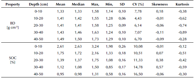
SD: standard deviation; CV: coefficient of variation; Max: maximum; Min: minimum
Source: Authors
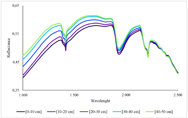
The average spectral signature for all soil samples grouped by soil depth is shown in Figure 2. The behavior shown by the spectral signatures at each sampling depth can also be qualitatively related to some of the soil properties. In the NIR, at wavelength ranges of 1 000-1 350 nm and 1 400-2 200 nm, spectral responses tend to be smoother and have a lower magnitude of reflectance in soils with a higher content of organic material (Poppiel et al., 2018). This is because organic matter affects the albedo of soils, which makes them reflect less light at higher levels of organic content (organic carbon) (Camacho-Tamayo et al., 2014). The spectral signatures obtained in this study showed a spectral reflectance according to these characteristics, as higher SOC contents were observed at lower sampling depths, which is consistent with the lower magnitudes of reflectance at a greater proximity to the soil surface.
BD and SOC modeling performance
The performance of the most accurate spectral models for BD and SOC is shown in Table 2. These were calibrated with 70% of the total signatures and validated with the remaining 30%. The BD spectral model turned out to be unrepresentative, reaching a RPD of 1,35 with an R2 equal to 0,41 during its validation. On the other hand, SOC showed excellent performance, reaching RPD and R2 values of 5,63 and 0,97, respectively.
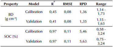
The underperformance obtained for the spectral model of BD has also been reported in other studies (Katuwal et al., 2020; Moreira et al., 2009). Particularly, the work by Moreira et al. (2009) consisted of 1 184 samples with BD values in the range of 0,45-1,95 g cm-3. They managed to validate models with R2 between 0,10 and 0,34 by applying different pretreatments to the spectral signatures. Meanwhile, Katuwal et al. (2020) achieved slightly higher performances, with R2 between 0,10 and 0,52 while working with a BD range of 1,02-2,01 g cm-3. BD is a soil property whose estimation through spectral signatures depends on the correlations that it may have with other attributes with recognized associations in the spectral range (Askari et al., 2015; Viscarra Rossel and Webster, 2012). For example, Al-Asadi and Mouazen (2014) coupled auxiliary variables such as water content, texture fractions, and organic matter with spectral models of BD in order to improve estimations, going from R2 values between 0,23 and 0,69 to a 0,70-0,81 range.
The level of performance obtained for the SOC estimations has also been reported in other works, corroborating the potential use of NIR spectroscopy for the prediction of this property (Jia et al., 2017; Nawar and Mouazen, 2019; Nocita et al., 2014). An example of this can be found in the large-scale study conducted by Liu et al. (2019), in which a model composed of 11 213 soil samples with a mean SOC content of 1,84% and magnitudes ranging from 0,02% to 9,96% achieved a validation R2 equal to 0,96 and a RMSE of 0,29%.
SOCS spectral estimation
The result of the product between BD [kg dm-3] and SOC [gC kg-1] is the volumetric SCOS [gC dm-3] (SCOSv), which was the value estimated from spectral models. The performance of the models calibrated via the established groups ranging from 10 to 300 samples is shown in Table 3. It was evidenced that, by increasing the number of samples used to calibrate the models, the RMSE decreased while the RPD and R2 increased. This bears out the fact that more robust estimation models can be achieved with more samples. The stabilization of these parameters occurs at around 90 samples for the calibration model, so this number was chosen as optimal for SCOS spectral modeling. However, it is worth highlighting that each of the models defined in Table 3 showed RPD and R2 values greater than 2,0 and 0,80 in the validation parameters.
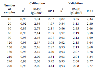
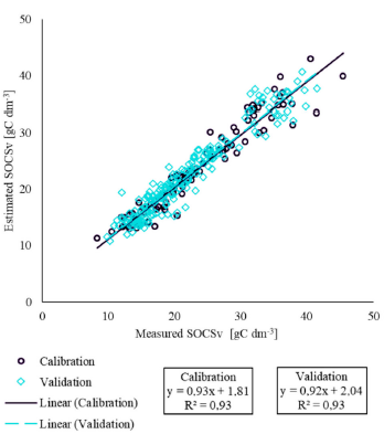
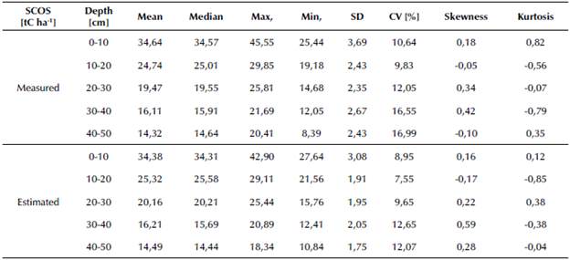
According to the RPD, the model made with the calibration group of 90 soil samples gave excellent estimates for SCOSv, with a RMSE of 2,12 gC dm-3 and a R2 of 0,93 (Figure 3). The calibration range for this model was 8,39-45,55 gC dm-3, while the range was 9,81-41,61 gC dm-3 for the validation group. The behavior of the measured and estimated SCOS in the soil profile is shown in Table 4. No large differences between the measured and estimated SOCS were evidenced. The datasets showed similar magnitudes regarding the mean and median, as well as for skewness, kurtosis, and the CV, which was in fact lower at each one of the sampling ranges (estimated vs. measured SOCS). The average content regarding the SOCS measured in the whole depth range of 0-50 cm was 109,28 tC ha-1. This value was 110,56 tC ha-1 for the estimated data.
A study carried out by Cambou et al. (2016) reported acceptable models regarding the estimation of SCOS from spectral signatures acquired in the field for a haplic luvisol, reaching R2 and RPD values of 0,70 and 1,80, respectively, for SCOSv values ranging between 7,90 and 27,70 gC dm-3. Part of the flaws in the estimation model of said research were attributed to the fact that the spectral signatures were collected by manually extracted auger soil cores that altered the natural structure of the samples. This, in addition to the fact that conventional laboratory analyses for BD and SOC were not performed on the soil samples from which the spectral signatures were collected (Cambou et al., 2016). On the other hand, Allory et al. (2019) compared the performance of models calibrated for urban soils using spectral signatures acquired in the field and in the laboratory. With a SCOSv range of 0,30-54,60 gC dm-3, a validation model was obtained with a RPD equal to 2,20 and an R2 of 0,78 for spectral signatures acquired in situ, while, for the laboratory-acquired spectra, the model parameters reported were 3,1 for the RPD and 0,89 for the R2. The performance improvement of the latter was attributed to the more stable measurement conditions in the laboratory, in comparison with those in the field.
For tropical volcanic soils that included andosols, cambisols, and ferralsols, Allo et al. (2020) calibrated models with spectral signatures obtained in the field and in the laboratory, obtaining better results in the validation of the model elaborated from signatures taken in situ (R2 = 0,91 and RPD = 3,29) when compared to the validation of the laboratory spectral model (R2 = 0,86 and RPD = 2,63). Allo et al. (2020) used a mechanical column auger to collect spectra in the field, allowing them to collect 30 signatures uniformly every 10 cm of the sampled soil column to establish an average signature for a single sample, achieving a closer representation of natural conditions. Doing this could have considerably improved the predictive ability of the model with spectra taken in situ vs. those acquired in the laboratory.
Given that the magnitudes of SOC and SCOS tend to increase at depths closer to the surface and decrease at lower depths in the soil profile (FAO, 2019; Stockmann et al., 2013), the Intergovernmental Panel on Climate Change recommends monitoring these organic C concentrations at least in the depth range of 0-30 cm (IPCC, 2019).
This recommendation is also motivated by the fact that the first 30 cm from the soil surface usually experience substantial changes in SOC due to management practices. Hence, the detection of variations in SOC reserves at this depth range could be noticed in shorter periods of time, depending on the activities carried out on them (Huang et al., 2019). In this regard, the oxisols of the Eastern Plains in the study area show a cumulative mean value of 78,85 tC ha-1 in the first 30 cm of soil depth, which, for estimated spectral data, equals 79,86 tC ha-1 and corresponds to approximately 72% of the total SOCS present in the profile considered.
SOCS spatial variation
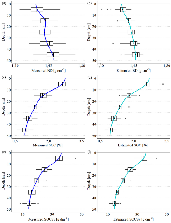
The vertical variation of the soil properties is shown in Figure 4. The splines allowed to estimate the value of soil attributes within each measured depth. Furthermore, the addition of boxplots to these diagrams aided in examining the similarity between measured and estimated data. At first glance, it can be noted that the resulting splines for BD have clear differences, which are attributed to the low representativeness of the spectral model. The interquartile range, as well as the whiskers of the boxplots, showed a considerable reduction for the estimated data in comparison with the measured values. The unrepresentativeness obtained in the spectral modeling for BD can be associated with the alteration of the structure of the soil samples prior to the signature acquisitions, as the soil samples were dried and sieved.
Source: Authors
Figure 4 Depth splines for standard laboratory-measured (a, c, e) and spectral estimated data (b, d, f)
Furthermore, the splines confirmed the excellent performance of spectral models for SOC and SOCSv. Even though a reduction can be perceived in the interquartile ranges of the boxplots of the estimated data when compared to those of the measured data, in general, the ranges of the whiskers of the estimated and measured data are similar. However, it can be pointed out that the loss of performance of the SCOS spectral model in comparison with the SOC one is due to the incorporation of the BD in the estimated variables, since this property could not be estimated directly with the same degree of representativeness.
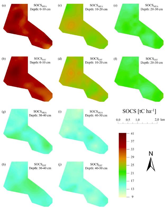
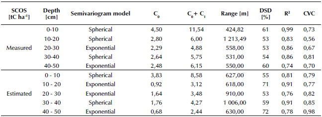
The results of the geostatistical analysis for the measured and estimated SOCS are shown in Figure 5 and Table 5. The semivariograms were adjusted to spherical and exponential models, which were the same for the measured and estimated data at every depth range except for 10-20 cm. Moreover, for each of the semivariograms in the five sampling depths, the nugget and sill values were lower for the spectral vs. the measured data. Therefore, it can be stated that the variance is lower in the estimated data. Lower nugget and sill values for the spectral data have also been reported by other authors (Araújo et al., 2015; Bonett et al., 2016; Camacho-Tamayo et al., 2017; Wetterlind et al., 2008). Among the sampling depths, the greatest variability of the SOCS was evidenced in the semivariograms at the closest range to the soil surface, which is consistent with the natural addition processes taking place in the study area.
Source: Authors
Figure 5 Interpolation surfaces of SOCS from measured (a, c, e, g, i) and estimated (b, d, f, h, j) data
The use of spectrally estimated data in the construction of semivariograms did not modify the spatial variation tendency of the SOCS, as was verified in the obtained models and the interpolation surfaces illustrated in Figure 5. DSD shows moderate spatial dependence for each of the sampling depths, which is also consistent for the spectral and measured data. In addition, most R2 and CVC values were above 0,70.
The geostatistical interpolation surfaces obtained from estimated and measured data showed a high degree of correspondence at each sampling depth. This is a positive indicator for approaching SOCS monitoring through spectral models, given that, once a sufficiently robust model is reached with adequate performance regarding the needs, the volume of information obtained could increase without the need to spend resources on conventional laboratory analyses, which is convenient for addressing soil studies in the context of climate change.
Conclusions
NIR spectroscopy allowed estimating, with a high degree of representativeness, the SOCS of oxisol in the study area. The results suggest that laboratory analyses for SOCS could be largely substituted or complemented by an approach involving spectral techniques in the NIR region. This work also showed that data derived from NIR models could be integrated into geostatistical evaluations for Colombian oxisols.

