ARTÍCULO ORIGINAL

Robust Design in Multiobjective Systems using Taguchi's Parameter Design Approach and a Pareto Genetic Algorithm

Diseño Robusto en Sistemas Multiobjetivo usando el enfoque de Taguchi de Diseño de Parámetros y un Algoritmo Genético de Pareto

Enrique Canessa^* , Gabriel Bielenberg, Héctor Allende

Facultad de Ingeniería y Ciencias. Universidad Adolfo Ibáñez. Av. Padre Hurtado 750. Viña del Mar, Chile.

^*Autor de correspondencia: teléfono:: + 56 32 2503752 , correo electrónico: ecanessa@uai.cl (E. Canessa)

(Received June 03, 2013; accepted May 12, 2014)

Abstract

We present a Pareto Genetic Algorithm (PGA), which finds the Pareto frontier of solutions to problems of robust design in multiobjective systems. The PGA was designed to be applied using Taguchi's Parameter Design method, which is the most frequently used approach by practitioners to executing robust design studies. We tested the PGA using data obtained from a real single-output system and from multiobjective process simulators with many control and noise factors. In all cases, the PGA delivered Pareto-optimal solutions that adequately achieved the objective of robust design. Additionally, the discussion of the results showed that having those Pareto solutions helps in the selection of the best ones to be implemented in the system under study, especially when the system has many control factors and responses.

Keywords:Parameter Design, Pareto genetic algorithms, multiobjective evolutionary algorithm

Resumen

Se presenta un Algoritmo Genético de Pareto (AGP), que encuentra la frontera de Pareto en problemas de diseño robusto para sistemas multiobjetivo. El AGP fue diseñado para ser aplicado usando el método de Diseño de Parámetros de Taguchi, el cual es el método más frecuentemente empleado por profesionales para ejecutar diseño robusto. El AGP se probó con datos obtenidos de un sistema real con una respuesta y de un simulador de procesos multiobjetivo con muchos factores de control y ruido. En todos los casos, el AGP entregó soluciones óptimas que cumplen con los objetivos del diseño robusto. Además, la discusión de resultados muestra que tener dichas soluciones ayuda en la selección de las mejores a ser implementadas en el sistema bajo estudio, especialmente cuando el sistema tiene muchos factores de control y salidas.

Palabras Clave:Diseño de Parámetros, algoritmos genéticos de Pareto, algoritmos evolucionarios multiobjetivo

Introduction

Robust design tries to adjust controllable input variables (control factors) of a system, so that its outputs stay as close as possible to their corresponding target values and with minimum variability, even in the presence of noise factors, which cannot be controlled [1, 2]. The most frequently used approach among practitioners to performing robust design is Taguchi's Parameter Design (PD) [3-9]. PD carries out this process in two stages. First it attempts to manipulate control factors to achieve minimum possible variability in the system's responses. Then it sets other control factors to locate the mean of the responses as close as possible to their corresponding target values. Given that performing experiments in real systems may require huge resources and imply long non-productive periods, PD makes extensive use of fractioning of experiments. This reduces the number of experimental conditions that must be run and the corresponding execution time [2, 10]. That is the reason why PD is so frequently used in real application of robust design [3-10]. Then, the manager takes into account time, costs and other economic factors associated with the setting of each of the control factors of the system to decide which solution to definitively implement [2]. If the system has many control factors with many possible levels and many responses that need to be simultaneously adjusted, that is a hard decision to make [1, 10-12]. Thus, to overcome some of the difficulties of applying PD to multiobjective systems with many control and noise factors, the work presented in [11] and [13] proposed the use of a Genetic Algorithm (GA). That GA automatically finds combinations of values for the control factors, which adequately locate the mean of the responses of the system as close as possible to their corresponding target values and with low variability. However, the manager still needs to select the best solution among the many ones delivered by the GA by trying to reach a compromise between variance reduction and mean adjustment [11, 13]. This is a rather complicated and time consuming analysis, especially when the system has many responses and needs to consider economic factors [13]. Thus, instead of manually dealing with the analysis, one could first compute a Pareto frontier with a Pareto GA (PGA) [14], which will show the compromise between variability reduction and mean adjustment for all of the responses. Then, the manager will use that frontier to consciously select a solution that efficiently deals with that balance, instead of just analyzing many solutions and choosing one that might not be a Pareto-efficient one. Thus, this paper presents an improvement to a previous GA [13], which consists in using a PGA that finds an approximate Pareto frontier for the problem of PD in multiobjective systems with many control and noise factors.

Other researchers have also explored the application of GA to robust design [15-20]. However, the present work differs from theirs in some important aspects. First, in general similar approaches have not used the application of PD and orthogonal arrays (OA) to the design and gathering of the experimental data. Given that the use of PD and internal and external OAs is the most frequently used method for conducting robust design studies by practitioners [3-10], the present work develops the PGA specifically for PD and OA. Second, much of previous work (see e.g. [16 - 19]) consists of particular tools applicable only to specific problems, and thus lack a more general view of robust design. Although previous research has its own merits, our work is readily generalizable to multiobjective systems with many outputs, control and noise factors, and uses Taguchis PD approach, the most frequently applied method in real studies of robust design [3-10]. Examples of such studies are the enhancement of copper refining methods to obtain a purer metal [1], an efficient scheduling of operators in a call-center [1], cost reduction in the processing of natural gas [21], improvement of end-milling operations to obtain a smoother surface of metal plates [22], to name just a few. Additionally, the present paper shows that the proposed PGA is robust against experimental design fractioning, resulting in further flexibility for applications in heavily constrained scenarios, which to our knowledge remains unaddressed in previous works.

Pareto Genetic Algorithm

Similar to the previous GA developed in [13], the proposed PGA represents the combinations of k control factors that may take S different levels (values) of a robust design experiment using an integer codification. Let f_ij be the factor j of chromosome l, with j = 1, 2, ..., k and l = 1,2, ..., N. Each f_ij can take the value of a given level of the factor j, i.e. 1, 2, ..., s. One chromosome (or solution) is expressed as a row vector (see Eq. (1)). The matrix representing the total population of solutions X will be composed of N chromosomes (see Eq. (2)).

Multiobjective Optimization Problem for a single-output system

In a single-output system, the experimenter needs to optimize only one response y. Thus, the PGA will deliver solutions that represent the optimal trade-off between variance reduction (minimize s² (X1)) and mean adjustment for y (minimize , and then the experimenter will select the solution that better meets his/her needs. In terms of a Multiobjective Optimization Problem (MOP) and following previous work [13], this problem can be expressed as follows (Eq. (3)):

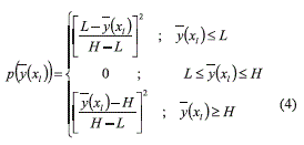
The restriction in (3) simply sets a lower (L) and upper tolerance limit (H), between which the mean of the response is acceptable. Following previous work [11, 13], the PGA uses the following penalty function for enforcing such limits (Eq. (4)):

Incorporating the penalty function (4) in (3) and defining expression (5):

the MOP can be stated as seen in expression (6):

The algorithm can then use φ₁ and φ₂ to establish the dominance relations between pairs of chromosomes (solutions). For two chromosomes, X₁ will dominate X₁ if and only if Eq. (7) is satisfied:

Multiobjective Optimization Problem for a Multiobjective System

A multiobjective system will have r responses (r = 1,…,R), so that now the PGA needs to decrease s²_r, ∀r and minimize , Mr. Thus, the PGA will use two desirability functions D₁ and D₂ for aggregating s²_r, ∀r and , respectively [13] [23, 24] (Eq. (8)):

Where is a vector with the mean of the responses of a solution x_l; and is a vector of the variances of that solution, with r=1,…, R, which can be seen in eqs. (9) and (10):

Each individual desirability d_ir (i = 1, 2; r = 1, 2,…, R) will be computed as suggested in [23, 24] by using expressions (11) and (12):

where a_ir and b_ir (i = 1, 2; r = 1, 2, … , R) are their least and most desirable cases respectively for the R responses as equation (13) shows:

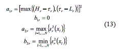
In expression (13), H_r and L_r are the upper and lower tolerance limits for response r, and Τ_r is the corresponding target value. Note that D₁ and D₂ in (8) and expressions (11) through (13) are defined so that larger values of D₁ imply that the mean of the responses are closer to their corresponding target values. Similarly, D₂ increases as the variance of the responses decreases. Thus, the MOP for the multiobjective case is stated as a maximization problem. Additionally, following the work presented in [23, 24], the PGA will use a penalty function P to penalize the infeasible solutions (those that provide a response beyond H_r or L_r) (Eq. (14)):

where each p_r is computed as expression (15) shows:

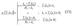
and c = 0.0001, which avoids p_r from becoming zero, and thus ensures that a non-zero P is calculated for a non-feasible solution (Eq. (14)) [24]. Finally, by defining φ₁ and φ₂ as shown by equation (16):

one can state a maximization problem for φ₁ and φ₂ (Eq. (17)):

Where chromosome x₁ will dominate x₂ if and only if eq. (18) is satisfied,

Multiobjective Evolutionary Algorithm

To solve the developed MOP we will apply the Multiobjective Evolutionary Algorithm (MOEA) Strength Pareto Evolutionary Algorithm 2 (SPEA2) [25, 26]. To apply SPEA2 to the MOP, we needed to make minor adjustments to the MOP already defined in subsection 2.1 and to the code of SPEA2. First, we restated expression (6) as a maximization problem, given that the code of SPEA2 is designed for maximization MOPs. Second, SPEA2 uses a truncation method for selecting its environment of possible solutions, which are kept in an external file of fixed size [25, 26]. However, in this case, the experimenter wants to compute as many feasible solutions as possible. Moreover, since in robust design the experimenter generally uses highly fractioned experimental designs [2, 10], he/she will have a reduced amount of data and thus, SPEA2 will not need to deal with a large number of solutions. Therefore, the present PGA uses an external file of variable size. Third, in the calculation of the φ₁ and φ₂ values for each chromosome (see Eq. (5) and (16)), the PGA needs to know the response/s corresponding to the experimental treatment, which each chromosome represents. However, remember that PD uses highly fractioned designs to reduce the size of the experiments [2, 10]. Hence, some of the treatments codified in some chromosomes might not have been part of the experiment that the manager conducted to gather the data. Thus, the PGA needs to estimate those responses. For estimating the mean and variance of the response for a non-tried treatment, the PGA calculates the main effect of each level of each control factor on both mean and variance. Then, for estimating the mean of a response, the PGA adds to the mean of all the responses of the experiment that was carried out, the corresponding main effects. For the variance, the PGA calculates a total variance considering all the replications of all the treatments tried in the original experiment and then the PGA adds to it, the corresponding variance main effects. Both procedures were successfully applied in previous GAs [13], and represent the usual form of estimating responses in PD [2]. Finally, we must note that the PGA uses a uniform crossover operator with probability p_c equal to 0.3 and a bit by bit (factor by factor) mutation operator with probability p_t equal to 0.05. Those operators and values are the same as the ones used in previous GAs with good results [11, 13]. The termination condition ofthe algorithm corresponds to reaching a fixed number of iterations, which was set at 15. The study tried larger values, but did not notice that the PGA obtained a better approximation to the Pareto frontier.

Application of the Pareto GA

To evaluate the performance of the PGA and also compare it to the previous GA (GA2) [13], two case studies were used. The first one corresponds to a real application of robust design. The second case study uses a multiobjective process simulator with four responses, ten control factors and five noise factors. This simulator is described in [11, 13]. For each of the test cases, PGA was run 30 times.

Results obtained for the single-output real system

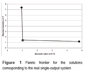
In this case, a robust design was carried out to adjust the width of the painted strip of a car painting system to a nominal width of 40.0 cm. In this process, it is very important to attain a specific width of the strip that is sprayed with paint. A narrow strip will leave parts of the car body with no paint and overspraying will result in waste of paint. This also means that the process should be very stable, i.e. the width of the painted strip should exhibit a small variability. In this study, the engineers and technicians identified four control factors each having three levels: type of spray gun used, speed of paint flow, fan airflow and atomizing airflow. The noise factors identified were three each with two levels: paint color, input air pressure and paint viscosity. The design of the experiment consisted of an orthogonal array L₉(3⁴) for the four control factors and a L₄(2³) for the three noise factors. More details and the data may be found in [27]. The Pareto frontier obtained by the PGA is presented in figure 1, which was consistently found in all the 30 runs performed. The points marked with a rhomb correspond to the solutions that define the frontier and were found by the PGA. The point marked with a triangle corresponds to one of the solutions delivered by the GA2 and selected as the best one, through a manual analysis [13]. That analysis consisted in calculating the mean adjustment and variance reduction attained by 17 solutions obtained by the GA2, and then selecting the one that presented a good compromise between both objectives. As can be seen, that solution coincides with one of the points of the Pareto frontier found by the PGA. Given the small size of the experiment, the manager can manually compute the Pareto Frontier and that best solution, which corresponds to the treatment (combination of control factors)A=2,B=3,C=1 and D=2 (chromosome x= [2 3 1 2]).

Given that the manually computed Pareto Frontier coincides with the one delivered by the PGA, it may be said that the PGA found a good approximation to the frontier. Table 1 1 shows the solutions that are part of the Pareto frontier found by the PGA. Having those figures, the manager can decide which of the solution best suits his/ her needs. If the manager takes into account only mean adjustment and variance reduction, most probably he/she will select solution 2-3-1-2, which is a good trade-off between both objectives. Now, if the manager considers economic factors, that decision is not so simple to make. However, the Pareto frontier will help the manager to consider the trade-off between variance reduction and mean adjustment, and economic issues. For this system, note that solution 2-3-1-2 and 1-3-3-3 achieve comparable standard deviations. Hence, any of the two, may be selected for achieving a low variability. On the other hand, although solution 1-3-1-3 achieves a good mean adjustment, it does not do well in variance reduction.

Now, according to the case study, factor A corresponds to the type of spray gun used, which can be of three types [27]. Also, the case study says that it is more expensive to use spray gun type 2 than type 1 [27]. Therefore, the manager may decide to implement solution 1-3-3-3 (A = 1 = spray gun type 1) rather than solution 2-3-1-2. This decision implies that it is tolerable and cost/ effective to achieve a width of the painted strip of 44.8 cm. [27] does not provide the figures to assess cost-effectiveness, but the analysis shows how having the Pareto frontier of solutions will help in making that type of decision.

Results obtained for the single-output complex systems

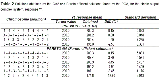
To test both GA's under a more complex situation, the study used the simulator described in detail in [13]. This process simulator has four responses, ten control factors and five noise factors. It also has interactions between control and noise factors. Those characteristics make the simulator similar to a real and difficult to optimize system [6]. The robust design for this situation considers using an inner array L₆₄(4¹⁰) for the ten control factors and an outer array L₁₆(4⁵) for the five noise factors. For the following case studies, the four responses of the simulator are optimized independently from each other, so that the PGA deals with four single-output systems. As in the previous case study, PGA was run 30 times for each test condition. For response one (y), table 2 shows the four best solutions obtained by analyzing the best 30 solutions found by GA2 and selecting the ones that are a good trade-off between mean adjustment and variance reduction. Additionally, table 2 presents the solutions that lie on the approximate Pareto frontier obtained by the PGA.

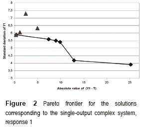
Figure 2 depicts the ten solutions showed in table 2. Comparing the solutions found by the PGA with those computed using the output of the GA2, figure 2 shows that only one of those solutions lies on the frontier and the other three are Pareto-inefficient Since the GA2 finds any reasonably adequate, not necessarily Pareto- efficient solutions; it is not surprising that some of the solutions found by the GA2 are Pareto- inefficient. Thus, although in the application of GA2, about 30 of its solutions were manually compared for selecting the best ones, the manager cannot be completely sure that those solutions will be the Pareto-efficient ones. Moreover, the manual analysis is prone to human errors, which could make the selection process even worse. That is why the PGA is so useful in this case: the manager will already have approximately Pareto- efficient solutions and then needs only to select among them, the one that best suits his/her needs.

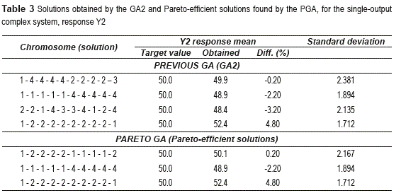
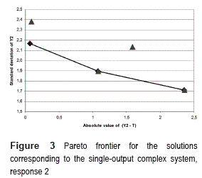
Similarly, table 3 presents the solutions for response two (y₂).

Figure 3 shows that two of the solutions, which were manually selected from the approximate forty obtained by the GA2, lie on the Pareto frontier. The other two are Pareto-inefficient. From table 3 one can also note that the PGA found a solution (1 - 2 - 2 - 2 - 2 - 1 - 1 - 1 - 1 -2), which adjusts the mean of the response as close to its target value, but with less variability, than the best solution in mean adjustment found by the GA2 (1 - 4 - 4 - 4 - 4 - 2 - 2 - 2 - 2 - 3).

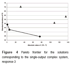
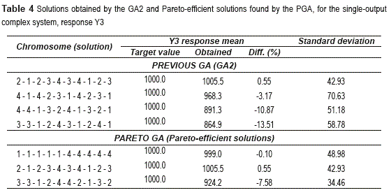
In the case of response three (y₃), the PGA also obtained three points of the efficient frontier. One of those points matches one of the manually selected solutions, which was chosen from the 30 solutions delivered by the GA2. This can be seen in figure 4.

The other three selected points are located rather far from the frontier. Table 4 shows the solutions along with the mean adjustment and standard deviation obtained by implementing each solution in the system simulator. The PGA found one new solution (1 - 1 - 1 - 1 - 1 - 4 - 4 - 4 - 4 - 4) that exhibits a better mean adjustment than the ones obtained by the GA2. However, in this case, the variance is higher.

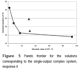
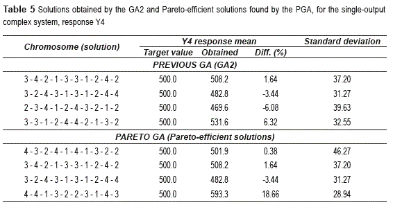
Finally, figure 5 and table 5 display the solutions for response four (y₄) The manual analysis selected four solutions among the fifty found by the GA2 and the PGA obtained four Pareto- efficient solutions. As can be seen in figure 5, two solutions of the GA2 coincide with the solutions of the PGA. In this case, the figures presented in table 5, show that the PGA found one solution (4 - 3 - 2 - 4 - 1 - 4 - 1 - 3 - 2 - 2) that adjusts the mean of response number four closer to its target value than the solutions obtained by analyzing the output of the GA2. However, the variance delivered by that solution is rather high. On the other hand, the PGA found the solution 4 - 4 - 1 - 3 - 2 - 2 - 3 - 1 - 4 - 3, which achieves the lowest standard deviation, but has the worst mean adjustment. Thus, the solutions obtained by the PGA allow the manager to assess the trade-off between mean adjustment and variance reduction. Note also that for the four responses, PGA consistently found the Pareto-efficient solutions in all the 30 runs performed.

Results obtained for the Multiobjective Complex System

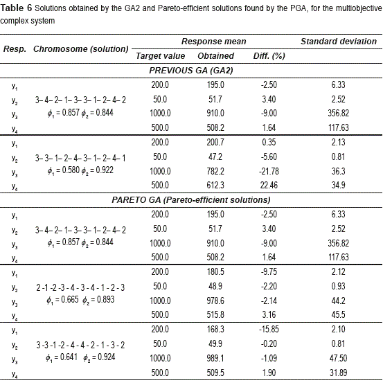
In this case the study used the same simulator and the same experimental design as before, but the PGA optimized the four responses at the same time. This means that the PGA is optimizing a four-dimensional multiobjective system. table 6 presents the solutions for this case.

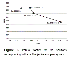
Table 6 shows the best solutions selected from about fifty of them found by the GA2, along with the three efficient solutions obtained by the PGA, which were consistently found in the 30 runs performed. For the solutions, table 6 reports the value of φ₁ and φ₂ which correspond to the aggregation of the desirability and penalty functions for the four responses (see expression (16)). For discussing the results, it is convenient to remember that φ₁ is related to mean adjustment and φ₂ is associated with variance reduction, where the PGA tries to simultaneously maximize those two figures, according to expression (17). Figure 6 shows the solutions, which were plotted using the corresponding values of φ₁ and φ₂.

In Figure 6, the points marked with a rhomb correspond to the solutions that define the frontier and were found by the PGA. The points marked with a triangle correspond to the solutions delivered by the GA2 and selected as the better ones, through a manual analysis [13]. Since in this case the PGA is maximizing and φ₁ and φ₂, the solution 3- 3- 1- 2- 4- 3- 1- 2- 4- 1 (φ₁=0.580 and φ₂=0.922) is Pareto-inefficient because it is dominated by solution 3 -3 -1 -2 - 4 - 4 - 2 - 1 -3 -2 (φ₁=0.641 and φ₂=0.924), and thus it is located to the left of the Pareto frontier. This frontier is not totally concave, as one should expect for a maximization problem. Given that the PGA was fed with a relatively small number of data points, one should expect to obtain a rough approximation to the Pareto frontier [28].

One of the solutions manually selected from the fifty best solutions obtained by the GA2 lies on that frontier. Note that the solution 2 -1 -2 -3 - 4 - 3 - 4 - 1 - 2 - 3, found by the PGA, may be a good compromise between mean adjustment and variance reduction. On the other hand, if a manager favors variance reduction, at the expense of mean adjustment, the solution 3 -3 -1 -2 - 4 - 4 - 2 - 1 - 3 - 2 might be the best to choose. On the contrary, if the manager favors mean adjustment, he/she might select the solution 3- 4- 2- 1- 3-3- 1- 2- 4- 2. In any case, looking at the values of the mean response for the four responses and their corresponding standard deviations in table 6, it can be seen that having the values of φ₁ andφ₂ and knowing which solutions are Pareto-efficient, helps in selecting the solution which better suits the manager's needs for mean adjustment and variance reduction. Additionally, remember that a manual analysis of about fifteen solutions delivered by GA2 was conducted for selecting the two solutions presented for that algorithm in table 6. It is easy to imagine how burdensome and prone to human errors it is to manually conduct that analysis for a system with many responses and control factors and many levels for each of them. Moreover, if the manager requires taking into account economic factors in his/her decision, that manual analysis becomes even harder. Thus, a graph like figure 6 and/or a table like table 6, may be of great assistance. That graph and table will show the manager the balance achieved by each solution regarding mean adjustment and variance reduction. Based on that, the manager can consciously select a solution that is cost/effective when factoring in the cost of implementing each solution.

Conclusions

The case studies involving the real system and the single-output and multiobjective process simulators showed that the Pareto GA (PGA) found a reasonable approximation to the Pareto frontier. That frontier contained solutions, which exposed the trade-off between the two objectives of robust design: adjusting the mean of the responses of a system to their corresponding target values and achieving a low variance for each response. Based on that frontier, the study analyzed the best solutions that were selected through a manual examination of between 17 and 50 solutions obtained by the previous GA2. In most cases, the Pareto frontier contained one or two of those solutions, but other solutions were not located nearby that frontier, i.e. were Pareto- inefficient. Since the GA2 finds good solutions, not the best and/or efficient ones, it is reasonable to have obtained that result. Moreover, the PGA automatically finds the Pareto-efficient solutions, whereas one has to manually evaluate many solutions obtained by the GA2 for selecting the best ones. Since that process is rather difficult and prone to human errors, especially when dealing with systems with many responses, control factors and levels for each factor, it is helpful to have the PGA. Additionally, in some of the single-output and multiobjective systems, the PGA found new solutions that achieved a closer adjustment of the mean of each response to their corresponding target values and attained an adequate low standard deviation of the responses. Note also that the performance of the PGA was consistently rather good under very different levels of fractioning of the experimental designs used to gather the data (e.g. case study one, which used a L₉(3⁴) for the four control factors and a L₄(2³) for the three noise factors; versus the other case studies that used a L₆₄(4¹⁰) for the ten control factors and a L₁₆(4⁵) for the five noise factors). This results in further flexibility for applications in heavily constrained scenarios.

Since the PGA seemed to work reasonably well in the case studies, it is meaningful to continue developing and improving it. One of such enhancements could be to try to achieve a better approximation of the Pareto frontier. Although robust design uses highly fractioned experimental designs, and thus the PGA works with a relatively small number of data points, the PGA could try to counterbalance that by using additional points calculated by response surface methodology (RSM) [29]. In this case, RSM may be applied for estimating the response surface of the system using the experimental data and then employing the response surface to calculate new points that will be used by the PGA. Second, the PGA can also consider economic factors in the calculation of the Pareto frontier. This might involve introducing desirability and penalty functions related to economic factors in the formulation of the MOP. By using equations similar to expressions (8) to (17), and considering the cost of each solution, one could begin to develop such MOP. Alternatively, the algorithm may incorporate a third objective that expresses the cost of each solution xt and state a three-objective MOP.

References

1. H. Allende, E. Canessa, J. Galbiati. Diseño de Experimentos Industriales. 1^st ed. Ed. Universidad Técnica Federico Santa María. Valparaíso, Chile. 2005. pp. 27-200.         [ Links ]

2. G. Taguchi. Systems of experimental design. 4^th ed. Ed. American Supplier Institute. Dearborn, USA. 1991. pp 397-511.         [ Links ]

3. G. Alexander. How to (almost) schedule innovation. Research Technology Management. Ed. Industrial Research Institute. 2002. pp. 31-40.         [ Links ]

4. D. Drickhamer. ''BASF breaks through with statistics''. Industry Week. June 2002. pp. 81-82        [ Links ]

5. C. Simms, J. Garvin. ''It's a black art: design of experiments switches on the light''. Managerial Auditing Journal. Vol. 17. 2002. pp. 65-71.         [ Links ]

6. R. Roy. Design of Experiments Using the Taguchi Approach. 1^th ed. Ed. J. Wiley & Sons. New York, USA. 2001. pp. 8-513.         [ Links ]

7. J. Cesarone. ''The power of Taguchi''. IIE Solutions. November 2001. pp. 36-40.         [ Links ]

8. J. Antony, F. Antony. ''Teaching the Taguchi method to industrial engineers''. Work Study. Vol. 50. 2001. pp. 141-149.         [ Links ]

9. K. Ballantyne, R. van Oorschot, R. Mitchell. ''Reduce optimisation time and effort: Taguchi experimental design methods''. Forensic Science International: Genetics Supplement Series. Vol. 1. 2008, pp. 7-8.         [ Links ]

10. S. Maghsoodloo, G. Ozdemir, V. Jordan, Ch. Huang. ''Strengths and limitations of Taguchi's contributions to quality, manufacturing, and process engineering''. Journal of Manufacturing Systems. Vol. 23. 2004. pp. 73-126.         [ Links ]

11. H. Allende, D. Bravo, E. Canessa. ''Robust design in multivariate systems using genetic algorithms''. Quality [ Quantity Journal. Vol. 44. 2010. pp. 315-332.         [ Links ]

12. S. Maghsoodloo, C. Chang. ''Quadratic loss functions and SNR for a bivariate response''. Journal of Manufacturing Systems. Vol. 20. 2001. pp. 1-12.         [ Links ]

13. E. Canessa, C. Droop, H. Allende. ''An improved genetic algorithm for robust design in multivariate systems''. Quality [ Quantity Journal. Vol. 42. 2011. pp. 665-678.         [ Links ]

14. C. Fonseca, P. Flemming. Genetic algorithms for multiobjective optimization: Formulation, discussion, and generalization. Proceedings of 5^th International 22. Conference on Genetic Algorithms, Morgan Kaufmann. San Francisco, USA. 1993. pp. 416-423.         [ Links ]

15. A. Kumar, A. Keane, P. Nair, S. Shahpar. ''Efficient genetic algorithm based robust design method for 23. compressor fan blades''. Proceedings of ASME IDETC/CIE Conferences on Design Engineering. Long Beach, USA. 2005. pp. 1-9.         [ Links ]

16. A. Hajiloo, N. Nariman-Zadeh, A. Moeini. 24. ''Pareto optimal robust design of fractional-order PID controllers for systems with probabilistic uncertainties''. Mechatronics. Vol. 22. 2012. pp. 788-801. Available on: http://dx.doi.org/10.1016/j. mechatronics.2012.04.003. Accessed: May 21, 2012.         [ Links ]

17. A. Jamali, A. Hajiloo, N. Nariman-zadeh. 2010. ''Reliability-based robust Pareto design of linear state feedback controllers using a multi-objective uniform- diversity genetic algorithm (MUGA)''. Expert Systems with Applications. Vol. 37. 2010. pp. 401-413.         [ Links ]

18. O. Koksoy, T. Yalcinoz. ''Robust design using Pareto type optimization: a genetic algorithm with arithmetic crossover''. Computers [ Industrial Engineering. Vol. 55. 2008. pp. 208-218.         [ Links ]

19. B. Forouraghi. ''A Genetic Algorithm for Multiobjective Robust Design''. Applied Intelligence. 27. Vol. 12. 2000. pp. 151-161.         [ Links ]

20. K. Hacker, K. Lewis. Robust design through the use of a hybrid genetic algorithm. Proceedings of ASME IDETC/CIE Conferences on Design Engineering. 28. Montreal, Canada. 2002. pp. 1-10.         [ Links ]

21. N. Yusoff, M. Ramasamy, S. Yusup. ''Taguchi's parametric design approach for the selection of optimization variables in a refrigerated gas plant''. 29. Chemical Engineering Research and Design. Vol. 89. 2011. pp. 665-675.         [ Links ]

22. J. Zhang, J. Chen, E. Kirby. ''Surface roughness optimization in an end-milling operation using the Taguchi design method''. Journal of Materials Processing Technology. Vol. 184. 2007. pp. 233-239.         [ Links ]

23.E. Del Castillo, D. Montgomery, D. McCarville. ''Modified desirability functions for multiple response optimization''. Journal of Quality Technology. Vol. 28. 1996. pp. 337-345.         [ Links ]

24. F. Ortiz, J. Simpson, J. Pigniatiello, A. Heredia- Langner. ''A Genetic Algorithm Approach to Multiple - Response Optimization''. Journal of Quality Technology. Vol. 36. 2004. pp. 432- 449.         [ Links ]

25. M. Laumanns, L. Thiele, E. Zitzler. SPEA2: Improving the Strength Pareto Evolutionary Algorithm. Technical Report 103. Computer Engineering and Networks Laboratory (TIK). Swiss Federal Institute of Technology (ETH). Zurich, Switzerland. 2001. pp. 1-21.         [ Links ]

26. M. Laumanns. SPEA2-The Strength Pareto Evolutionary Algorithm 2. Swiss Federal Institute of Technology (ETH). Zurich, Switzerland. 2008. Available on: http://www.tik.ee.ethz.ch/~sop/pisa/ selectors/spea2/?page=spea2.php. Accessed: October 10, 2012.         [ Links ]

27. W. Vandenbrande. Make love, not war: Combining DOE and Taguchi. ASQ's 54th Annual Quality Congress Proceedings. Indianapolis, USA. 2000. pp. 450-456.         [ Links ]

28. C. Coello, G. Lamont, D. Van Veldhuizen, D. Evolutionary Algorithms for solving Multi-Objective Problems. 2^th ed. Ed. Springer Science+Business Media. New York, USA. 2007. pp. 233-282.         [ Links ]

29. R. Myers, D. Montgomery. Response surface methodology: process and product optimization using designed experiments. 2^nd ed. Ed. J. Wiley [ Sons. New York, USA. 2002. pp. 536-605.         [ Links ]