


 Inglês (pdf)
 Artigo em XML
 Referências do artigo
 Enviar este artigo por email
 Citado por SciELO
  Citado por Google
  Similares em
SciELO
Similares em
SciELO  Similares em Google
 Permalink
1. Introduction
1.1. Motivation
Multidimensional signals are an important class of signals which are widely used in diverse applications such as medical imaging[1, 2], spectral remote sensing for target detection, classification or unmixing of substances[3, 4] and spectral imaging[5]. In these applications, the signals exhibit a multidimensional structure, where each dimension has a physical meaning e.g., space, time, frequency, wavelength. As a consequence, these signals contain more information about a phenomenon, and their processing is expensive in terms of computational complexity compared to unidimensional signals. In this regard, a tool in signal processing to deal with this problem is the sparsity. A signal is sparse if its energy is concentrated in just a few number of its coefficients[6]. Natural signals and images are not commonly sparse, but they could have a sparse representation by using an appropriate basis or dictionary[7, 8]. The sparse representation of signals has long been exploited in signal and imaging processing for various tasks such as compression, denoising[9-10], and compressive sensing[8-11]. The most popular dictionaries to obtain sparse representations are the ones obtained through the use of the Discrete Cosine Transform (DCT), and the Wavelet transform[12]. This kind of dictionaries are called analytical dictionaries given that they model the signals through the use of mathematical functions, which allow fast and implicit implementations to obtain useful representations. However, these representations are as accurate as the underlying model allows it, because the model needs to cope with the complexity of the natural phenomena, and in reality these models are inclined to be simple[13]. The learning dictionaries approach exists since they fit a given model, in particular with more accuracy, thus extracting information directly from the data itself.
1.2. Related work
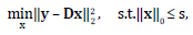
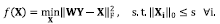
In the literature, there exists two main models for the sparse representation of signals named the synthesis and the analysis models[14]. The synthesis sparse coding problem is the most popular and it states that a signal y ϵ ℝ n can be represented in a dictionary D ϵ ℝ nxd as a linear combination of a few elemental columns, called atoms[9-13]. This means that the signal can be obtained as y = Dx, where ϵ ℝ d is the sparse representation, with║ x ║0 « d, where ║·║0 is the l 0 quasi-norm that counts the non-zero entries of a vector. In this model, the sparse representation x can be obtained by solving the optimization problem in Eq. (1) [6-15]
 (1)
(1)
Where s is the desired sparsity level of the representation, ║·║2 is the l
2 norm  , and s « d. Finding the solution to this problem is non-deterministic polynomial-time hard (NP-hard). Despite of this, there are algorithms that can find a solution in polynomial time, under certain conditions[6-15]. On the other hand, the analysis model states that a signal y can be represented in an analysis dictionary Ω ϵ ℝmxn via inner products with its rows, referred as analysis atoms, with ║Ωy║0 = m-1, where Ωy ϵ ℝm is sparse, and l are its number of zeros, called the co-sparsity[16]. In contrast to the synthesis model, this model allows obtaining the representation just by multiplying the signal y with the analysis dictionary Ω.
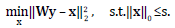
The sparse representation models can be adapted to train dictionaries from training signals. There exist various state-of-the-art works that explore dictionary learning using the synthesis approach[17-18], and the analysis approach[19-21], but most of them have to solve a non-convex problem where finding a solution is NP-Hard. As an alternative to the two previously mentioned models, there exist the so called transform model[22]. This model states that a signal y can be approximately represented in a sparse way in a transform basis W ϵ ℝmxn, as Wy = x + e, where x ϵ ℝm is sparse with ║x║0 «m, and e is the representation error in the transform domain. This model is a generalization of the analysis model with Ωy exactly sparse and, unlike the analysis model, it allows the sparse representation x not to be constrained to lie in the range space of the transform W[22], which implies that the transform model is more general than the analysis model. Assuming that  the problem of obtaining a sparse representation x, given a sparsity level s for a signal y with a known transform basis W can be formulated as in Eq. (2)
 (2)
(2)
The corresponding solution to the problem in Eq. (2) is obtained by hard thresholding Wy, i.e. by retaining its s largest coefficients. In comparison, the synthesis and analysis models, need to solve the sparse coding problem, dealing with NP-hard problems.
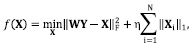
The transform model in Eq. (2)( can be generalized in order to obtain a sparsifying transform W from a matrix of training signals Y ϵ ℝnxN with sparse representation X, such that each column represents a training signal, with N as the number of training signals. Constraining the model to obtain a square transform can be formulated by minimizing the error given by  , where W ϵ ℝnxn, X ϵ ℝnxN[22], and by expressed it as in Eq. (3)
 (3)
(3)
Where X is column-sparse, and ║·║F is the Frobenius norm  Note that, in Eq. (3) the log det W term penalizes the transforms with small determinants, helping to obtain a full rank transform W, thus avoiding trivial solutions, such as those composed by repeated rows. Similarly, the
  term helps to control the condition number of the transform W[22].
In this paper, we propose an algorithm to learn sparsifying transforms from multidimensional signals based on the transform model given in Eq. (3). The proposed algorithm exhibits better performance than analytical transforms for sparse representations, and in contrast to synthesis or analysis dictionary learning strategies, the transform model allows approximating WY by a column-sparse matrix X, leading to a simpler, faster and cheaper implementation.
2. Proposed algorithm
In this section, an algorithm is proposed to solve the problem in Eq. (3). This algorithm alternates between two stages, a sparse coding stage in which the problem seeks to find sparse representations X of the training signals Y, fixing the transform basis W; followed by a dictionary update stage, where the transform W is updated by fixing the just found sparse representation X. The stages are detailed as follows:
2.1. Sparse coding step
In this step Eq. (3) is solved by fixing the dictionary W. This can be written as Eq. (4)
 (4)
(4)
An easier problem than that in Eq. (4) can be obtained by relaxing the ℓ0 quasi-norm constraint to the ℓ1 norm, moving it to the objective function using Lagrange multipliers. The resulting optimization problem can be formulated as in Eq. (5)
 (5)
(5)
Where η is a regularization parameter, and ║·║1 represents the ℓ1 norm. The relaxed problem in Eq. (5) can then be solved through a soft thresholding as presented in Eq. (6)
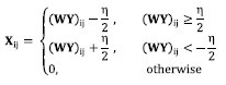 (6)
(6)
where the subscripts i, j index the matrix entries. An alternative solution to the optimization problem in Eq. (4) can be obtained by hard thresholding, that is, by maintaining the s largest coefficients in each of the columns of WY[22].
2.2. Dictionary update step
This step involves solving Eq. (3) by fixing the previously found sparse representation matrix X. This solution can be modeled as the unconstrained non-convex optimization problem in Eq. (7)
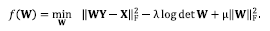 (7)
(7)
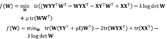
A solution to problem in Eq. (7) can be found using algorithms such as the steepest descent, the conjugate gradient, among other mathematical optimization algorithms[23]. This work uses a conjugate gradient algorithm with backtracking line search given its faster convergence compared with steepest descent. To ease the process of finding the gradient of Eq. (7), we rewrite Eq. (7) as in Eq. (8),
 (8)
(8)
by using the fact that 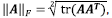 where “tr(.)” represents the trace. Expanding Eq. (8) it is obtained Eq. (9) as,
 (9)
(9)
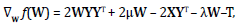
where the last line follows by the property of the trace being a linear mapping. Therefore, the gradient of the function f (W) in Eq. (9) is given by Eq. (10),
 (10)
(10)
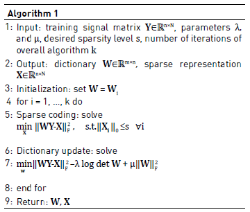
by using the fact that  For the conjugate gradient algorithm iterations, various stopping criteria can be selected, but based on empirically results, it is used a fixed number of iterations, due to the fast convergence of the algorithm. An initial W transform with positive determinant must be chosen for the algorithm to work. The proposed algorithm is summarized in Algorithm 1.
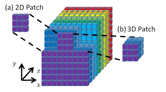
Solving the sparse coding and dictionary update problems could become computationally expensive for large signals. Therefore, we propose to use small-size non-overlapping patches to reduce the computational burden of the algorithm. The training signals Y are then proposed to be vectorized patches of a certain three-dimensional image. Two setups were considered using non-overlapping patches taken from the three-dimensional images: two-dimensional (2D) and three-dimensional (3D) patches. The use of patches entail dictionaries that can adapt to high correlated training signals with similar sparsity, thus allowing more flexibility. An sketch of the patch extraction procedure is depicted in Figure 1. The two-dimensional patches consist of taking a predefined number of pixels along two dimensions with the remaining dimension fixed. The three-dimensional patches consist of taking a predefined number of pixels along the three dimensions of the images.
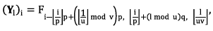
Having an image as a three-dimensional array Fϵ ℝ NxMxL, it can be written in an indexed form as F i,j,k , where i, j and k indexes are the two spatial and the spectral coordinate, respectively. The patches size in the spatial coordinate x is defined as p, and in the spatial coordinate y is defined as q. The vectorized 2D patches of the three-dimensional array are formulated as the l th column of the training signal matrix Y as given in Eq. (11)
 (11)
(11)
For i = 0, 1, … ,pq - 1,  , where
  , and “mod” is the modulo operation. For the 3D patches approach, a similar process is followed but additionally defining the patch size in the spatial coordinate z as r. The vectorized 3D patches of the three-dimensional array are then formulated as the lth column of the training signal matrix Y as in Eq. (12)
 (12)
(12)
For i = 0,1, … , pqr - 1, 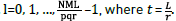 .
.
3. Experiments
Several experiments with real multidimensional images were conducted to show the benefits of the proposed algorithm. Experiments were performed using three test multidimensional signals shown in Figure 2: an hyperspectral image (HSI) composed of a section of a Lego scene with spatial resolution of 128 x 128, with 24 spectral bands[24]; a magnetic resonance image (MRI) composed of a resized scene of a head scan, property of the U.S. National Library of Medicine[25], with dimensions 128 x 128 x 32; and a computerized axial tomography scan (CAT) image of a human thorax acquired with a computed tomography scanner Toshiba Aquilion 64 with dimensions 128 x 128 x 60.
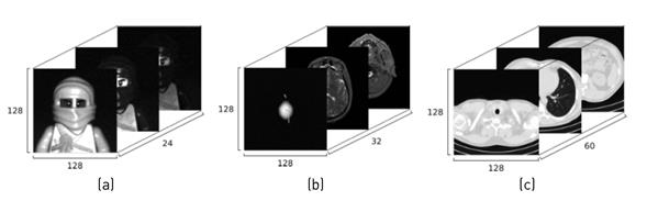
Figure 2 Multidimensional training images. (a) HSI image with size 128 x 128 x 24, (b) MRI image with size 128 x 128 x 32, (c) CAT image with size 128 x 128 x 60
The hyperspectral images are three-dimensional images consisting of large amounts of two dimensional spatial information of a scene across a multitude of spectral bands (wavelengths). In contrast, the magnetic resonance images are three-dimensional images with three spatial coordinates captured with a magnetic field and pulses of radio waves. Similarly, the computerized axial tomography images are three-dimensional images with three spatial coordinates captured using X-rays, to obtain projections at different angles with respect to an object of interest.
The size of the patches used for the 2D case was set to be 8 x 8 pixels, and for the 3D patches was set to be 8 x 8 x 4 pixels. As used in common image processing applications[26], the mean of the patches (DC values) are removed prior to processing; that is, only mean-subtracted patches are processed, but the means are added back later only for display purposes. The proposed algorithm was run for a fix number of 20 iterations. The sparsity level of the signals was varied between 15% and 50%. For the sparse coding step, although soft thresholding is convex, the hard thresholding scheme was used due to the overhead to adjust the parameter η in Eq. (6). For the transform update step, the conjugate gradient algorithm was used and run for a fixed number of 10 iterations. The initial transform Wi was chosen to be the 2D DCT matrix. An estimate of the training matrix is calculated as  and used to reconstruct the training multidimensional image. This output image is compared against the input multidimensional image in order to measure the quality of the results reached by the algorithm. The best parameters λ and μ in Eq. (10) were found for each experiment by try-and-error running the algorithm multiple times.
In particular, three sets of experiments were performed to test the proposed algorithm using the three multidimensional images shown in Figure 2. In the first experiment, we perform a sensitive analysis of the regularization parameters λ and μ, seeking for the best values, since their correct selection highly impacts the final result. In the second experiment, we compare the performance of the proposed algorithm using either 2D and 3D patches with the best regularization parameters found in Experiment #1, against analytical transforms such as DCT and the identity, and the state of the art dictionary learning algorithm K-SVD [17]. In order to quantify the reconstruction quality of the multidimensional test images from the learned dictionary W, the peak signal-to-noise ratio (PSNR) metric was calculated. The third experiment analyzes the concentration of the non-zero values of the signals after being represented on the attained dictionaries. The higher the concentration of the non-zero values, the better the representation dictionary.
3.1. Experiment #1: Regularization parameters search
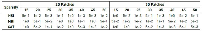
Figure 3 shows the performance of the algorithm for different sparsity settings between 15% and 50%, versus the value of the parameters λ and μ, in terms of the PSNR of the reconstructed images attained from the estimation of the training matrix  . The regularization parameters were varied in the interval (10-5, 101), and where set to be equal (λ = μ). The latter setting empirically proved to maintain a good leverage between the terms in the objective function. The parameters which yield the highest PSNR for each image are shown in Table 1, and these were chosen to be used for the rest of the experiments.
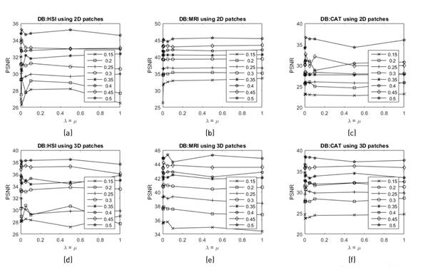
Figure 3 Sensitive analysis of the regularization parameters λ and μ for the different multidimensional test images in terms of PSNR, using 2D patches and 3D patches, respectively for (a-d) HSI image, (b-e) MRI image, and (c-f) CAT image
3.2. Experiment #2: Comparison with state-of-the-art methods
In order to test the accuracy of the proposed algorithm to create sparsifying dictionaries, we compare it against analytical dictionaries obtained through the DCT and the identity matrix. Moreover, we compare the proposed method against the widely-used state of the art dictionary learning algorithm K-SVD, which has shown to be reliable. Figure 4 summarizes several simulations that were performed varying the sparsity level of the signals to be represented by the dictionary. Note that the best regularization parameters were used for the proposed algorithm using either 2D or 3D patches, as given in Table 1.
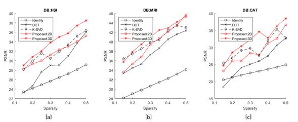
Figure 4 Comparison between the proposed method, the DCT and identity analytical transforms, and the state of the art dictionary learning K-SVD algorithm for different sparsity levels, in terms of PSNR for the three multidimensional test databases
In Figure 4, it can be observed that the analytical transforms generated from the identity matrix and the DCT perform worse than the dictionary learning algorithms, being the DCT dictionary the closest one. Comparing the dictionary learning methods, it can be seen that the K-SVD algorithm performs relatively well, since its attained PSNR results are sandwiched between the behavior of the proposed algorithm using 2D and 3D patches. Remark that the use of 3D patches entails the best PSNR performance overall, confirming the assumptions that 3D patches represent better the correlations within high dimensional signals. In addition, Figure 4(a), 4(b) and 4(c) show that the compared algorithms seem to behave similarly no matter the number of slices of the multidimensional images being tested.
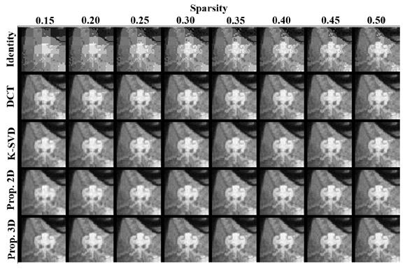
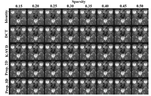
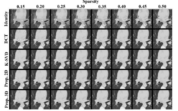
To evaluate the spatial quality of the reconstructed images based on the estimation of the training matrix, a comparison along the 2D spatial domain against the original test multidimensional images was made. Figures 5, 6 and 7 show zoomed versions of a single slice for each multidimensional test image, respectively, comparing the five methods listed in Figure 4, using different target sparsity levels. It can be confirmed from these figures that the proposed method using the 3D patches scheme performs best overall, for the three multidimensional images tested. Note however, that close results are attained by using the 2D patches scheme and the K-SVD algorithm.
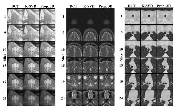
In Figure 8, a comparison of the footprints of 6 different slices along the third dimension of the three test databases is shown, in order to analyze the performance of the best analytical (DCT), the K-SVD and the best proposed method (using 3D patches). It can be observed from the figure that each algorithm performs consistently along the third dimension, with the K-SVD and the proposed method attaining the best quality.
3.3. Experiment #3: Concentration of the non-zero coefficients (sparsity)
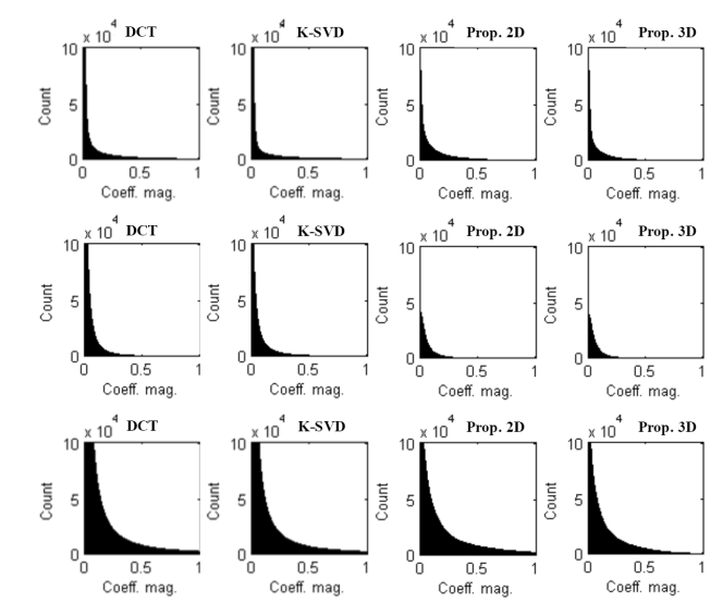
This experiment analyzes the concentration of the non-zero values of the signals after being represented on the trained dictionaries. For each multidimensional sparse representation in each dictionary, a threshold is applied to remove the values close to zero, in order to observe the non-zero coefficients with higher magnitudes; that is, the most representative coefficients. Table 2 shows a comparison of the number of non-zero coefficients attained after applying a threshold to the normalized magnitudes lower than 0.03. It can be observed that the number of non-zero coefficients is lower for the learned dictionaries than that of the DCT, and between the learned dictionaries, the proposed method using 3D patches attain the sparsest representations.
Table 2 Number of non-zero coefficients with normalized magnitude greater than 0.03, obtained by representation of the databases using the 4 dictionaries
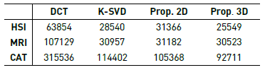
Figure 9 shows the count of the non-zero coefficients for the 4 used dictionaries after being applied to the three multidimensional databases. It can be observed from the figure that the analytical transform generates representations with more non-zero coefficients and with small magnitudes (near to zero) than the representations obtained through the use of the trained dictionary. This means that the representations obtained through the trained dictionaries are better for sparsifying multidimensional signals than the analytical transforms considered.
4. Conclusions
An algorithm for learning sparsifying transforms of multidimensional signals has been proposed in this manuscript. The proposed algorithm alternates between a sparse coding step solved by hard thresholding, and an updating dictionary step solved by a conjugate gradient method. Two variations of the algorithm using 2D and 3D patches were shown to process the multidimensional signals adequately, in terms of quality of the reconstruction for different test databases. The proposed algorithm was compared against analytical transforms such as the DCT, and the state of the art K-SVD dictionary learning algorithm. The proposed algorithm using 3D patches showed to have in general a better performance for the representation of the multidimensional images tested in this paper, both in terms of PSNR of the reconstructions and in terms of concentration of the non-zero elements, that is, the proposed method entails better sparse representations.

