


 Inglês (pdf)
 Artigo em XML
 Referências do artigo
 Enviar este artigo por email
 Citado por SciELO
  Citado por Google
  Similares em
SciELO
Similares em
SciELO  Similares em Google
 Permalink
1. Introduction
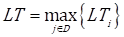
Increasing competition in today's global market has forced enterprises to configure and evaluate their supply chain (SC). Generally speaking, a SC is a network whose vertices represent different stages that perform different tasks such as the procurement of components, the assembly of products, and the delivery of products to customers. Each stage in the SC network often has several options for accomplishing its task, e.g. one stage may have the task of acquiring a component and the options are represented by the different suppliers from which the component could be supplied; every option is differentiated by its time and cost. Deciding what option should be used at each stage in order to minimise the CoGS and products' LT is known as SC design [1].
In recent years, many companies such as Dell Computers [2], Procter & Gamble [3], and Hewlett-Packard [4] have realised that to provide products with lower cost and shorter periods of time, they have to evaluate and design the structure of their SC continuously. According to [5], an optimum design decreases the cost by 10% and the service time is reduced by 40%. Despite these benefits, the SCD problem is not an easy task since there might be multiple suppliers that could supply each component, many manufacturing plants that could assemble each product, and many ways in which the product could be delivered to the customer.
Therefore, the problem is to determine: from which supplier should each component be obtained, where will each product be assembled, and which transport mode to use to deliver products to customers the complexity of the problem increases by the fact that the selected options that perform the stages must minimise the production cost (PC) and delivery time (DT), at the same time, for a family of products represented in a generic bill of materials.
In this paper, the SC representation proposed by [6] is used. There are I stages (i=1,2,…,I ) and every stage has J i possible options (j=1,2,…,J i ) that can perform it. Every option j i has a cost (c ij ) and time (t ij ) associated, and for any pair of options j and j' that can perform the stage i their cost and time have the following relationship: c ij > c ij’ ( t ij > t ij’ or c ij ( c ij’ ( t ij ( t ij’ .
The SCD problem, as stated in this paper, is a classical combinatorial optimisation problem in which the solution is not based on a sequence but on the selection of variables that ‘best’ perform the objective functions, i.e. the solution of this problem is to select the subset of options (or variables) which minimises the PC and DT. According to this, the number of solutions or possible SC designs is  .
.
The primary intent of this research is to develop an algorithm based on a new nature-inspired swarm-based meta--heuristic called Intelligent Water Drop (IWD) to solve the SCD problems as stated in this paper. In IWD, there are R rivers (r =1,2,…,R) , each one with Dr drops (d =1,2,…,Dr), and every drop designs an SC, thus a solution is sd=(LT, PC).
As our proposed algorithm minimises two objectives, we applied the Pareto optimality criterion to the solutions to determine which solutions are ‘better’ than others; thus, a set of non-dominated solutions are computed. A solution of this kind is one in which any improvement in one objective can only take place if at least one of the other objectives worsens.
Many techniques and approaches have been used to solve the SCD problem. These techniques include mathematical programming, metaheuristics, and agent technology. In relation to mathematical programming, the SCD problem as stated in this work has been studied in [7]. Those approaches use standard operation of dynamic programming to solve a single-objective mixed-integer problem (MIP) that just minimises the PC given that an amount of safety stock is placed on the stages. In [8] the same problem is solved using genetic algorithms in order to reduce the computational time. In[9], the same MIP model is solved by means of a fuzzy model in which the cost and lead time for every stage have three values: the pessimistic, the expected, and the optimistic cost and lead time. A genetic algorithm is used to solve the fuzzy model.
In [10], the SCD problem is formulated as a multi-objective stochastic MIP model in which the uncertainty is represented by means of a demand forecast. This model is solved by ε-constraint method, and branch and bound techniques. Objectives are to maximise profit over the time horizon, maximise the demand satisfaction and minimise the financial risk.
A MIP model is develop in [11] to solve a three-echelon SC that comprises manufacturing plants, warehouses, and retailers. In this approach, the aim is to locate several warehouses in potential places to minimise the total transportation cost from manufacturing plants to warehouses and from warehouses to retailers. The model has manufacturing plants and warehouse capacity constraints. The quantity of products sent by the manufacturing plants to a particular warehouse must be the same quantity as that sent by the warehouse to all the retailers being served. The above model was extended in two ways [12]. First, not only the transportation cost is included but also the assembly and fixed costs of a warehouse and manufacturing plant. Second, not only the warehouses must be located but also the products must be allocated to manufacturing plants. In [13], the same three-echelon SC was studied but the production, material handling, and importing costs are included. In addition to the constraints of production and warehouse capacity and material balance, there are material flow constraints which guarantee that material only flows from a manufacturing plant to a warehouse if there is a link that joins them. In the above approach, the capacity of the facilities and the number of manufacturing plants and warehouses are fixed values. A MIP model in which the capacity and number of facilities are variables is stated in [14], thus the complexity of the problem is increased. This model minimises both the cost of transportation among plants, warehouses, and customers as well as the cost of operating the manufacturing plants and warehouses that were located. The results of this model are the number of manufacturing plants and warehouses and their location as well as the capacity level of the facilities. The MIP model includes constraints of capacity and material balance.
The novelty in this work is to compare the performance of the proposed IWD algorithm with exhaustive enumeration for an instance size that the optimum Pareto set can be computed. Moreover, the model in this paper considers more than one option to perform a stage, contrary to what is done in the aforementioned proposal. In relation to the application of IWD to the SCD problem, there is no published attempt to solve the bi-objective SC configuration by means of IWD as shown in recent surveys specialised in SC design problem [15-17].
2. Problem formulation
2.1. Intelligent Water Drop algorithm and Pareto criterion
The IWD metaheuristic is a novel swarm-based algorithm which imitates the natural process that takes place between the water drops and the river bed. This metaheuristic was first proposed to solve the Travelling Salesman Problem with results that showed the algorithm converges fast to optimal solutions and finds goods and promising solutions [18]. Then, the multiple knapsack problem and the n-queens problem were solved with comparable results than those computed with other metaheuristics. Recently, IWD has been used to solve some problems in engineering, such as the trajectory planning in aerial vehicles [19], irrigation systems design [20], and economic load dispatching [21].
The basic idea embedded in IWD is that water drops follow an ideal straight line from their origin to their destination (that is usually a lake, a sea, or a bigger river) because of the gravitational force. This is not possible since there are obstacles and barriers that force drops to look for an unblocked path. An important barrier in a path is the amount of soil in it, hence the drops look for paths that have neither obstacles nor soil.
Every water drop reaches its destination because of two properties: the amount of soil it carries and the velocity that allows drops to carry more soil from the bed of the river. Therefore, three important rules are: a) the faster the speed of the water drop, the larger the amount of soil it carries, b) the velocity of the water drop increases on paths with less soil, and c) when a drop selects a path, it is selected based on the amount of soil in the path.
In this way, the first water drops “clean” the river of soil, allowing subsequent water drops to travel faster in the river. Notice that water drops and paths both have soil. In artificial water drops d, the problem is represented by a network G={V,E} in which the following steps take place: a) while d is in a vertex of V, it selects the following vertex to go based on the probabilistic decision rule that is a function of the soil over the path that links the two vertices, b) the velocity of d is updated once it has moved forward, and c) the amount of the soil over the link is modified. When d has reached its destination, it has generated a sequence of vertices in V. The sequence generated by d is compared with the best-so-far sequence to determine if there is an improvement in the objective function. After that, a global soil update process is carried out, thus an amount of soil in the path that represents the best-so-far sequence is removed.
As our proposed algorithm minimises two objectives, LT and PC, the concept of Pareto Optimality Criterion is applied to determine which solutions are better than others; thus, a set of non-dominated solutions is computed. A solution of this kind is one in which any improvement in one objective can only take place if at least one of the other objectives worsens. Hence, a solution s={s1,…,sk} (in our case s1 = PC and s2 = PC) dominates another solution s’={s’1,…,s’k} represented by  , if and only if
 The non-dominated solutions form the solution set represented by
  where
where  is the feasible space.
2.2. Mathematical representation of formulation
The mathematical representation used in this paper is modified from [22]. Hence, we modelled the SC as a graph G={V,E} where the set of vertices represents the supply, manufacturing, and delivery stages (i), thus V = {1,2,…,i,…,I }. The set of edges represent the relationships between two stages. These relationships could be: a supply and a manufacturing stage, two manufacturing stages, or a manufacturing and a delivery stage, thus E={(1,2),(1,i),…,(i,i’)}. The subset of delivering stages is defined as D( V. This is important since the products' demand is generated in those stages, μ i given that I ( D.
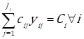
Every stage i has different options j which can perform the stage, j( i. To select an option to perform a stage, a binary variable is used. This variable is defined as follows: y ij = 1, if the option j performs stage i. Otherwise, y ij = 0. Hence, the PC is defined by Eq. (1) which computes the total cost of all the products that are delivered to customers during the company's interval time of interest (.
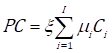 (1)
(1)
μ
i
is the demand at stage i, defined as  and C
i
is the cost of the selected option at stage i see Eq. (2).
and C
i
is the cost of the selected option at stage i see Eq. (2).
 (2)
(2)
Formally, the SCD problem is formulated as a bi-objective mixed-integer programming model. The two objectives to minimise are Eqs (1) and (2), subject to Eqs (3) to (7).
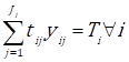
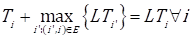
The SC is designed when Eqs (3), (4), and (6) are solved, i.e. when the values of all the binary variables are known y ij as well as when the time (T i ) and cost (C i )$ of the stages are set. Eq. (5) computes the lead time for all the stages and Eq. (7) is to make sure y ij can only take the values of 0 or 1.
 (3)
(3)
 (4)
(4)
 (5)
(5)
 (6)
(6)
 (7)
(7)
2.3. Proposed IWD algorithm
As said before, a solution or SC configuration generated by the water drop d is presented by s
d
= (LT, PC) and the solution set contains all the non-dominated solutions SS = {s
1
,…, s
d
,…}. Therefore, s
d
= (LT, PC) dominates s’
d
= (LT’, PC’), if  To add a solution to the SS, the last condition must be proved for every solution generated by each water drop.
Once, every drop  (r=1,..,R) has computed a s
d
(d=1,…,D
r
), the concept of Pareto Criterion is applied to all the solutions. Therefore, every river r computes a solution set SS
r
and the last one is returned as the problem solution set, i.e. SS
R
=SS.
(r=1,..,R) has computed a s
d
(d=1,…,D
r
), the concept of Pareto Criterion is applied to all the solutions. Therefore, every river r computes a solution set SS
r
and the last one is returned as the problem solution set, i.e. SS
R
=SS.
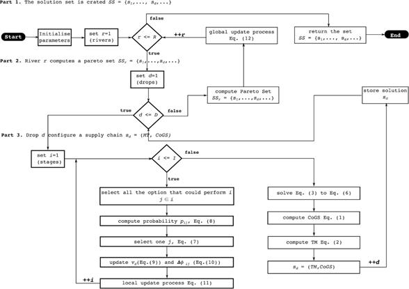
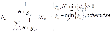
The soil is represented by φ ij , i.e. φ ij is the quantity of soil deposited in option j that can perform the stage i, φ d is the quantity of soil carried by water drop d, and v d is its velocity. The proposed algorithm is divided into two parts (see Figure 1). In the first one, each single drop d configures the SC visiting all the stages. While a water drop is at stage i, the drop computes the probability p ij which is a function of the soil at every option. As shown in Eq. (8), when the minimum amount of soil in all the options is less than or equals to zero, the minimum amount is subtracted from the value of φ ij to select the option with the least possible amount of soil.
 (8)
(8)
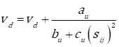
θ is a very small constant to avoid divisions by zero. As a rule, the higher the value of p ij , the higher the probability of selecting option j to perform i. Once an option has been selected, the velocity of the water drop is updated by Eq. (9) and the increments of the amount of soil are computed using Eq. (10) (a, b, and c are constants). The local update process (in which the soil is modified at the stage and at the water drop) is carried out by Eq. (11), where ρ n ((0,1) is the local updating parameter.
 (9)
(9)
 (10)
(10)
 (11)
(11)
Notice that the time τ ij spent in option j at stage i is a function of the two objectives to minimize. At the end of this first part, the SC is configured and the second part of the algorithm is run.
In the second part, the amount of Cost of Goods Sold is computed using Eq. (1) as well as the lead time using Eq. (2).
When all the drops have built a solution, the Pareto optimality criterion is applied to all the solutions and the non-dominated ones are added to the solution set. Finally, the soil in every stage that belongs to a solution in the Pareto set is updated per Eq. (12), where ρ w is the global updating parameter used to ‘delete’ a fraction of the soil over the selected options j.
 (12)
(12)
3. Experimentation
A notebook supply chain example is adapted from [22]. The example involves a supply chain producing two types of products, namely Grey Notebook and Blue Notebook. The former satisfies both US and export demand while the latter is only sold to the US market. The two products require similar components and sub-assemblies until a point
of differentiation where either the Grey or Blue cover is included. The tree structure, in Figure 2, shows the components and operations that are required to manufacture the products and deliver them to markets. For each product, four types of components are required to produce a circuit board assembly, which is then assembled with an LCD display, a metal housing, a battery, and various other components to produce a notebook subassembly. The notebook subassembly is then integrated with either the Grey or the Blue cover to make up the final products.
According to Figure 2, the size of the set of vertices is 17, thus V={1,2,…,17} and the set of edges is: E ={(1,5), (2,5), (3,5), (4,5), (5,10),$ $ (6,10), (7,10), (8,10), (9,10),(11,13), (10,13), (10,14), (12,14), (13,15), (13,16), (14,17)}. The subset of delivering stages is D={15, 16, 17}. There are ten supplying stages (i=1, 2, 3, 4, 6, 7, 8, 9, 11, 12) and five manufacturing stages (i= 5, 10, 13, 15).
The data used to run the algorithm is provided in Table 1. Accordingly, the problem has 24,576 possible solutions. To test the proposed algorithm, we created three instances. The first one is the one described above, hence instance 1 has the three Notebooks and three delivering stages. The second instance includes only the Grey Assembly and two delivering stages and the instance 3 includes the Blue Assembly and one delivering stage.
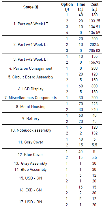
The proposed algorithm was tested creating one thousand drops (D = 1'000) and run twice. In run one, we used thirty rivers (R=30) and in the second run ten rivers (R=10) were created. In every run, the initial soil at all the options is 10'000 and the initial velocity at every drop is 200. The other parameters are set as follows: a = c = 1, b=0.001, and ρ n , ρ w = 0.01.
4. Results
As the proposed algorithm is based on a new metaheuristic, we compared the results returned by it to the optimum Pareto set computed by exhaustive enumeration. In Figure 3(a), the whole solution space, for instance 1, is shown. Notice that the PC ranges from 1.73 x 10⁶ to 7.41 x 10⁶ but most of the solutions are between 1.73 x 10⁶ and 2 x 10⁶. Therefore, the solutions with PC within this range are plotted in Figure 3(b). The aim of the first experiment was to define the number of rivers with which the algorithm returns the closest solution set to the optimum Pareto set. We proved graphically and analytically that the algorithm seems to return a similar solution set to the optimal one when the number of rivers is increased. In order
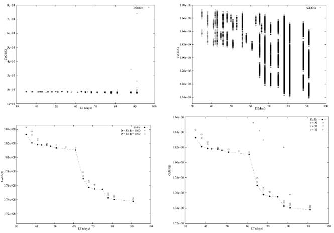
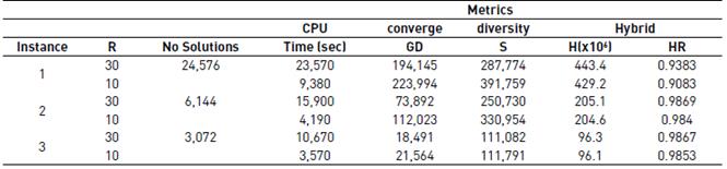
In Table 2, the value of each metric for every instance is summarised. The GD computes the average distance between two solution sets, that generally one of them is the optimum Pareto set. The smaller the value of GD, the closer the solution set to the optimum one. For instance 1, the GD=194,145 when 30 rivers are created (R=30), but when R=10 the GD=223,994. Therefore, it seems that the algorithm converges to the optimal Pareto set when $R=30$. As shown in Figure 3(c), 82% of the solutions computed when R=30 have lower PC than those computed when R=10, thus we can conclude that when R=30 the proposed algorithm returns a solution set similar to the optimum one.
In Figure 3(d), the solution sets computed by rivers r=10, r=20, and r=30 are plotted for instance 1 (remember that r =1,…,R). The objective of this is to show how every river computes a solution set closer to the optimum one, thus we computed the GD for every river, i.e. GD10=2,256,227, GD20=214,085, and GD30=194,145. According to the GD metric, we can conclude that the algorithm tends to converge to the optimum Pareto set.
The metric S that measures the diversity of the solution set states that the smaller the S, the more evenly apart (or spaced) the solutions. This metric is important since we are interested in finding solution sets uniformly distributed over the solution space, i.e. S measures the dispersion and extension of the solution sets. As seen in Table 2, the S=287,774 when R=30 and S=223,994 when R=10, thus the solution set computed when R=30 is more uniformly distributed over the solution space as shown graphically in Figure 3(c).
The hybrid metrics called Hypervolume (H) and H Ratio (HR) are related to the coverage area of a solution set in relation to the solution space, i.e. H and HR add the rectangle areas bounded by a reference point. For instance 1, the reference point is LT = 91 and CoGS=187,039,500, hence the value of H is greater when R=30, i.e. about 94% of the area is covered by the solution set when R=30. On the other hand, when R=10 just 9% of the area is covered. According to the values of GD, S, H, and HR in instance 1, we concluded that the best solution set computed by our proposed algorithm is when thirty rivers are created.
A similar analysis can be carried out in instances 2 and 3. As shown in Table 2, the values of the metrics when R=30 outperform the values of the same metrics when R=10 but in the H and HR in which their values are similar. It means that in instances 1 and 2 the area, covered by either of the solution sets, covers about 98% of the solution space area.
In relation to the CPU time, the maximum CPU time is about 23 seconds that are spent by our algorithm when R=30 and instance 1 was solved. Notice that instance 1 is the one with the largest solution space, thus we can conclude that the larger the instance and the larger the number of rivers, the longer the CPU time as shown in Table 2. We used a Lenovo ThinkPad T520 computer with an Intel Core i5 processor at 2.50GHz and 4Gb in RAM memory.
5. Conclusions
In this paper, we applied a new metaheuristic to the SC configuration problem. To the best of our knowledge, there are no published attempts to solve the SC configuration problem using this metaheuristic. The aim of this piece of research is to test the Intelligent Water Drop metaheuristic and to prove graphically and analytically the performance of the proposed IWD-based algorithm by using convergence and diversity metrics.
We proved that our algorithm returns a solution set similar to the optimum Pareto set when the number of rivers is set to 30 instead of 10 for the proposed Notebook SC used as experimental application. We were able to compute the solution space for the bigger instance (the one which contains the Blue and Gray Notebook) and we concluded that the algorithm converges to the optimum Pareto set according to the Goal Difference Metric and the returned solution set is evenly spaced. The hyper volume ratio or percentage of the area covered by the returned solution set is at least 91%. Hence, the proposed algorithm returns a solution set similar to the optimum one.

